Novel LPV-based Control Approach for Nonlinear Physiological Systems

Novel LPV-based Control Approach for Nonlin- ear Physiological Systems

Gy¨orgy Eigner

Physiological Controls Research Center

Research and Innovation Center of ´Obuda University Kiscelli u. 82, H-1032 Budapest, Hungary

eigner.gyorgy@nik.uni-obuda.hu

Abstract: The current paper introduces a novel controller design approach dealing with the control of affine Linear Parameter Varying (LPV) systems using the abstract mathematical properties of the LPV parameter space and classical state-feedback design. By the designed controller structure the parameter dependent LPV system mimics a given selected reference LTI system reaching given performance specifications originally prescribed for the reference LTI system. Further, the actual feedback gains are calculated by comparison to the reference control gains - thus, realizing a ”relative control”. The method is demonstrated on given nonlinear biomedical problems with simulation results under MATLAB.

Keywords: LPV model; Affine LPV; qLPV; Physiological control

1 Introduction

Nonlinear controller design is a challenging task even using current increased com- putational power. Although the physical reality is mostly nonlinear, the most widely used controller design approaches are based on linear controller design methodolo- gies providing particular solutions around the favorable operating range of the origi- nal systems. In the last decade, different controller design solutions appeared trying to describe and handle the whole operation range of the nonlinear systems based on optimization, iteration or else and they exploited the possibilities of the increased numerical calculation capacities [1].

The recently developed Robust Fixed Point Transformation (RFPT)-based controller design [2] uses inverse kinematics and dynamics to accurately approximate the sys- tem to be controlled and formalize the control task as a fixed point problem. If the conditions are satisfied through the convergence of Cauchy series in the Banach- space the controller adapts itself to the requirements of the system along the prede- fined performance specification [2].

Significant direction is the usage of the Lyapunov stability theorems combined with Linear Parameter Varying (LPV) methodology, as the conditions of the stability are

defined as Linear Matrix Inequalities (LMI) and the solutions, namely, the appropri- ate controllers can be calculated through advanced LMI-optimization tools [3]. This direction is represented by the Tensor Product (TP) transformation based controller design which originates from the Fuzzy theorem and uses the LPV-LMI optimiza- tion methods [4].

The current research work focuses to an other direction, namely, how can be used the mathematical properties of the LPV parameter space in controller design re- garding the classical state feedback control in such a way that the completed con- troller structure handles the LPV system and through the original nonlinear system.

This approach does not require convex LMI optimization neither inverse kinemat- ics, however, it can provide global stability.

The paper is structured, as follows: first we introduce the affine LPV systems and the classical state feedback approaches; after, we present the proposed novel con- trol scheme; then the method is demonstrated via a nonlinear biomedical problems;

finally, we conclude the results of the research.

2 Affine LPV Configuration

The affine LPV configuration originates from the Linear-Time Invariant (LTI) and Variant (LTV) systems. The classical state-space representation of an LTI system can be described as:

˙

x(t) =Ax(t) +Bu(t) +Ed(t)

y(t) =Cx(t) +Du(t) +D₂d(t) , (1)

whereA(t)∈R^n×nis the state matrix,B(t)∈R^n×mandE(t)∈R^n×lare the control and disturbance input matrices,C(t)∈R^p×nis the output matrix,D(t)∈R^p×mand D2(t)∈R^p×l are the input and disturbance feed-forward matrices. Thex(t)∈Rⁿ, u(t)∈R^m,d(t)∈R^lvectors are the state, control and disturbance input vectors.

Similar to LTI systems, the parameter dependent affine LPV systems can be de- scribed easily with their general state-space representation:

˙

x(t) =A(p(t))x(t) +B(p(t))u(t) +E(p(t))d(t)

y(t) =C(p(t))x(t) +D(p(t))u(t) +D₂(p(t))d(t) . (2) In this case, each matrix is a function of the parameter vectorp(t)∈R^k, which is a k-dimensional real time function and the elements of it are the scheduling variables - the preliminary selected functions of the given nonlinear system [3]. Thus, this configuration allows to handle the nonlinear system as a linear one by hiding the nonlinearity of the system inside the scheduling variables. Hence, by the use of LPV systems linear controller design methodologies can be applied on the nonlinear systems itself.

Among different representation of LPV systems, in the affine case the scheduling parameter is a function of the a state / states and these dependencies can be described

as follows [3]:

A(p(t)) =A₀+

k i=1

∑

p_i(t)A_i B(p(t)) =B₀+

k i=1

∑

p_i(t)B_i

E(p(t)) =E₀+

k i=1

∑

p_i(t)E_i C(p(t)) =C₀+

k i=1

∑

p_i(t)C_i

D(p(t)) =D0+

k i=1

∑

pi(t)D_i D2(p(t)) =D2,0+

k i=1

∑

pi(t)D_2,i

. (3)

3 State Feedback and Gain-Scheduling Control

The idea of optimal state feedback control for LTI systems originates from the 1960s when the cost function based optimization appeared in modern control engineering.

Over decades, different cost functions and feedback gain calculation techniques ap- peared like quadratic regulation, energy minimization, time minimization or track- ing error minimization, etc. [5]. Regarding to LPV systems the first generation of gain scheduling control techniques were developed in the late 1990s [6, 7].

In case of state feedback control, the control signal occurs in the following form:

u(t) =−Kx(t) , (4)

where K∈R^m×n is the feedback gain matrix. K can be designed via different iteration-based methods. For example, in case of Linear-Quadratic (LQ) control, the control input of (4) minimizes the following cost function [8]:

J(u) = Z _∞

0

x^TQx+u^TRu+2x^TNu

dt , (5)

and the optimal gain K can be calculated by solving the control algebraic Ricatti equation [8]:

A^TX+X A−(X B+N)R⁻¹(B^TX+N^T) +Q=0

K=R⁻¹(B^TS+N^T) . (6)

The optimalK gain provides better control performances through pole-placement of LTI systems. In general, this configuration modifies the open-loopA_open state matrix intoA_closed=A_open−BK via (4). The poles of the characteristic equation can be calculated, as follows:

|Iλ−A+BK|=0 . (7)

In gain-scheduling control, which is a natural choice in case of affine LPV system, the optimal gain becomes parameter dependent [6]:

u(t) =−K(p(t))x(t) . (8)

The class of p(t)dependent controllers of (8) are similar with the class of p(t) dependent system of (2). Since, the continuous controller design is impossible,

the reasonable choice is to divide thekdimensional parameter space into different slices. Hence, different controllers have to be designed for each slice and these con- trollers can handle the occurring LTI systems inside these slices. The drawback is the high computational capacity, complex switching schedule (as p(t)varies over time) and the necessary advanced methods providing global stability.

Instead of this natural, however sometimes unmanageable configuration, the poly- topic model configuration and polytopic controller design spread out in control en- gineering [3, 9–11].

In politopic cases, the number of necessary controllers are reduced. If, the parameter space is handled as a vector space and the occurring LTI systems (”system trajec- tory”) are inside a given region of the vector space, a convex hull can be designed, which wraps the system trajectory. As a result, it is enough to design specified number of controllers to the determining point of the p-space. Thus, if the con- vexity properties are fulfilled, the resulting controller (as convex combination of the designed controllers) can handle each occurring LTI system inside the poly- tope [10, 11]. The benefits of these methods are the drawbacks at the same time: the necessary deep mathematical knowledge and understanding, high computational ca- pacity. The global stability is only particularly true, i.e. if the system trajectory does not exit from the convex hull (the value of p(t)cannot be higher or lower than the predefined values) [11, 12].

4 Novel, Specific Control Scheme

We have previously investigated the opportunities of using the mathematical prop- erties of the parameter space in order to define norm-based performance markers for LPV systems and examined the general properties of models used in diabetes researches [11]. However, these properties can be observed in large number of physiological systems, as well:

• Input(s) are not affected by nonlinearities and do not have direct inputs-outputs connection (DandD₂are persistent in time and zero matrices)

• Output(s) are not affected by nonlinearities

• Since the nonlinearities do not affect the inputs and the outputs, it is not nec- essary to select their elements as scheduling parameters, which means that BandCare independent from the parameter vector p; moreover, these are usually time-independent

• The nonlinearities only appear in the state matrixA(p(t))regarding to the nonlinear system dynamics, nonlinear cross effects and nonlinear coupling;

the patient variabilities mostly occur in the elements ofA.

The necessity, which originally brought to life the LPV methods and theories was to handle the nonlinear systems as linear ones. Thus, each element of the time- dependent and nonlinearAshould be selected as scheduling variable.

In our previous study [11], we have shown that every parameter dependent LPV sys- tem can be equivocally determined by the belonging parameter vector if the above statements are fulfilled. In other words, each p parameter vector (a point in the parameter space) belongs to an underlying LTI system S(p), further, eachS(p)is equivocally determined by its correspondingpparameter vector.

4.1 Investigated LPV Model Class

Our investigation focuses on LPV systems that have parameter dependent elements only in theirA(p(t)), as follows:

˙

x(t) =A(p(t))x(t) +Bu(t) +Ed(t)

y(t) =Cx(t) +Du(t) +D₂d(t) . (9)

If the parameter vector is persistent in time, the belonging parameter dependent LPV system can be simplified to an LTI system. Moreover, the vary of p(t)realizes the system trajectory, which consist of infinite number of LTI systems. In this case, each points in the parameter space equivocally determines an underlying LTI sys- tem. This property allows to define different norms in the parameter space on the parameter vectors, however, most of them can be interpreted on the underlying LTI system.

In this study, we deal with this specific model class and the proposed controller design method is valid on this particular group of models (mostly true in case of physiological systems).

4.2 Mathematical Background

Definition 1. Similarity of matrices [13]: A quadratic, n×n matrix A is similar to a matrix B, if an invertible C matrix exists that A=C⁻¹BC. Notation: A∼B.

The definition above has wide range of applications. Two of them can be found in the following theorems [13, 14]:

Theorem 1. Similarity invariance of the determinants of matrices: If A∼B, then

|A|=|B|.

Proof. LetA∼B, namely,A=C⁻¹BC. Then|A|=|C⁻¹BC|=|C⁻¹||B||C|=|B|, since|C||C⁻¹|=1 [13].

Theorem 2. If A∼B, then the characteristic polynomials of the matrices and thus, the eigenvalues and the geometric and algebraic multiplicities of the eigenvalues of the matrices are the same.

Proof. Let A∼B, namely, A=C⁻¹BC. Then A−λI =C⁻¹BC−λC⁻¹IC= C⁻¹(BC−λIC) =C⁻¹(B−λI)C, namely,A−λI∼B−λI[13].

These mathematical tools can be used to define eigenvalues equality rules for state feedback systems.

4.3 The Completed Feedback Gain Matrix

Let us define the compact form of (9):

x(t)˙ y(t)

=

A(p(t)) B E

C D D₂



 x(t) u(t) d(t)



=S(p(t))



 x(t) u(t) d(t)



 , (10) whereS(p(t))∈R(n+p)×(n+m+l). Whenpis persistent in time, (10) simplifies to a LTI system, which is represented bySof (11).

x(t)˙ y(t)

=S



 x(t) u(t) d(t)



 . (11)

Each LPV system is dependent from the parameter vector p(t), which may vary in time. As we mentioned earlier, this variation realizes a system trajectory S(p(t)) in the parameter space, which consist of infinite number of LTI systems. These LTI systems appear over time, during the variation ofp(t). The only difference be- tween the occurred LTI systems are the different belonging parameter vectors, if the aforementioned requirements - each nonlinearity causing and time variant terms and variables have to be selected as scheduling parameter in order to avoid underlying differences, the nullspace problem, etc. [11] - are fulfilled.

From state feedback design point of view, without gain scheduling or other ad- vanced techniques that would mean the need of infinite number of optimal gains to handle the occurring LTI systems (in continuous time), which is obviously im- possible. However, if we want to apply the linear state feedback controller design techniques on the given LPV system, we can utilize this property, namely, the dif- ference between the occurring LTI systems are only the values of the belonging parameter vectors.

In order to embed the ”difference” into the controller scheme, we applied the re- sults of our previous study [11]. In this study, we concluded that it is possible to use 2-norm based difference interpreted on the space of the parameter vector to de- fine dissimilarities between LTI systems, which belong to given parameter vectors.

For example, in case of two pointsaandb in the parameter space represented by

”persistent” parameter vectors, the 2-norm based difference among these is:

e=||p_a−p_b|| . (12)

This difference marker allows the description of the difference between arbitrary points in the parameter space, in other words, the dissimilarities among different belonging LTI system (e.g. in the above mentioned case the dissimilarity between S(p_a)andS(p_b). Moreover, it is possible to usee(t)as a function of time, when we describe the difference between a reference pointp_{re f}and thep(t)and of course the dissimilarity between the belonging underlying LTI systems,S(p_{re f})andS(p(t).

In the followings a 2Dparameter space example is presented: having two schedul- ing variables p(t)∈R². During the operation of the system, the p(t)varies over time from p_act(t₀)top_act(t_n). It is possible to describe the 2-norm based difference

between the reference point p_{re f} and actual parameter vector p_act (and actual dis- similarity betweenS(p_{re f})andS(p(t))bye(t).

S(pre f) S(pact(t0))

S(pact(tn))

S(pact(tp)) e(t_p)

p₁(t) p2(t)

Figure 1

2Dexample of the interpretation of the 2-norm based difference between a reference point (reference system) and the actualp(t)(actual LTI systemS(p(t))).

Let us define a reference point in the parameter spacep_{re f}, which serves as the ref- erence parameter vector andSre f as its corresponding LTI reference system. Conse- quently classical state feedback design can be applied onSre f. Generally, the goal of controller design in such methodologies is to provide optimal feedback gains as a result of an integral optimization process. The appearing optimal feedback gain has to stabilize the system, and to reach better properties for the system to be controlled.

This should be done by the new poles of characteristic equation. Let us consider that K_{re f} is an eligible and optimal gain for theS_{re f} LTI system. In this case, the modi- fied state matrix of the state-feedback reference system will beA(p_{re f})−BK_{re f}and the eigenvaluesλre f can be calculated via solving the characteristic equation:

|Iλ_{re f}−(A_{re f}−BK_{re f})|=|Iλ_{re f}−A_{re f}+BK_{re f}|=0 . (13) In the parameter space, each underlying parameter dependent LTI systemS(p)is unequivocally determined by its belonging parameter vector p. If, the dissimilar- ity between the parameter dependent LTI systems can be described by the 2-norm based difference of the parameter vectors (as we have seen earlier), then it is possi- ble to use this connection to define such kind of unique, completed state feedback controller, which is designed for the reference LTI systemS(p_{re f}); however, it can deal with each occurring LTI system S(p(t))during operation. Moreover, if this completed controller can provide stability and good performance criteria for the ref- erence systemS(p_{re f}), it can provide the same properties for each occurringS(p) (and the LPV system S(p(t))). On the other hand, that means that, if we have a nonlinear system, we can transform it to an LPV system and with this approach, we can design a controller handling this LPV and in ultimate sense, the nonlinear system itself.

First of all, we consider that the LPV system is in the form of (10); thus, only the state matrixA(p(t))is parameter dependent. Let consider the closed-loop system matrix as follows:

A(p(t))−B(K_{re f}+Ke(t)) , (14)

wheree(t)is the 2-norm based difference between thep_{re f} andp(t)andKm×nis a continuously calculable gain. At this point, two main considerations are needed.

The first, that this configuration has to provide the stability, namely, the state matrix (14) of the newly defined closed-loop system should have eigenvalues with negative real parts. The second, this criteria can be satisfied, if we apply a specific form of the above defined Theorem (1)-(2).

LetA_{re f}+BK_{re f}∼A(p(t))−B(K_{re f}+Ke(t)), which means that the eigenvalues of the two matrices are equalλ(p_{re f}) =λ(p(t))at∀p(t), ifλ(p(t))is the eigenval- ues of(A(p(t))−B(K_{re f}+Ke(t))). This is only possible, if the similarity trans- formation matrix is theIn×nunity matrix. Namely,A_{re f}−BK_{re f} =I⁻¹(A(p(t))− B(K_{re f}+Ke(t)))I, i.e. the introduced completed gain has to provide the ”smoother”

similarity, but also the ”strict” equality criteria. Shortly, the proposed completed feedback gain K_{re f}+Ke(t)has to provide the equality of not just the eigenvalues λ(p_{re f}) =λ(p(t)), but also the equality of the matrices, as well:

A_{re f}−BK_{re f}=A(p(t))−B(K_{re f}+Ke(t)) . (15)

4.4 Consequences, Controller Design and Limitations

Let us consider that p(t)can be measured or estimated. In this case, the only un- known in matrix in (15) isK. By rearranging (15), theKcan be calculated at every

p(t):

K=B⁻¹(A_{re f}−BK_{re f}−A(p(t)) +BK_{re f})

e(t) =B⁻¹(A_{re f}−A(p(t)))

e(t) (16)

In this way:

A(p(t))−B(K_{re f}+Ke(t)) =

A(p(t))−B K_{re f}+B⁻¹(A_{re f}−BK_{re f}−A(p(t)) +BK_{re f})

e(t) e(t)

!

, (17)

such a controller structure appears, which can provide that the LPV systemS(p(t)) is going to behave as the feedback controlled LTI reference system S(p_{re f})itself, regardless from the actual value of p(t). Shortly, the LPV system will mimic the feedback controlled reference LTI system.

Figure 2 demonstrates the completed control loop in compact form - which is neces- sary to realize this idea in practice. Since, we considered that p(t)can be measured or estimated, the 2-norm based difference is available at any time.

At this point, we can summarize the main steps which are needed in order to realize the proposed controller design method:

S(p(t))

K(p_{re f}) +Ke(t)

z(t) x(t)

k.k₂

p(t)

p_{re f} - y(t) r(t) u(t)

-

Figure 2

Feedback control loop with completed gain

1. Realize and validate the LPV models in appropriate form (from the original nonlinear model),

2. Select the reference pointp_{re f}, which determinesS(p_{re f})reference system in accordance to the needs of reality; namely, the selection of such a reference LTIS(p_{re f})system is needed, which can provide the best operating results from the given application point of view.

3. State feedback controller design via linear controller design method in order to realize the optimalK_{re f} gain for theS(p_{re f})system.

4. Design of the eligible controller scheme, including the appropriate form of (16).

5. Realize of the control environment.

Through the above mentioned points, the controller design is possible and easy to handle. This novel method may provide another controller design possibility then gain scheduling or LPV-LMI based approaches, but have limitation as well:

1. In this point, we summarized the considerations so far, which are needed in order to use this controller design approach: the nonlinear system should be given in form of (10) or has to be transformed to this term; only theA(p(t)) can be parameter dependent in (10);p(t)should be measurable or estimable;

S(p_{re f})should be a well selected reference LTI system from the given appli- cation point of view. Each nonlinear system which is state-space represented, can be transformed to the form of (10), if the nonlinearities are connected to the selected state variables.

2. The invertibility ofBis a key point. Generally, Bn×mis not a square matrix and occasionally contains dependent linearly columns, as well. Here we have three cases: (i)Bis square matrix and invertible; (ii)Bis not a square matrix, however, does not contain linearly dependent columns; (iii)Bis not square matrix and does contain linearly dependent columns. In the first (i) case,B is invertible and (16) can be used to calculateK. For the second (ii) case, if Bis not a square matrix, but linearly independent, the left hand side matrix multiplication ofBwithB^T can be a solution. In this manner, the completion

of (15)-(16) is necessary, as follows:

A_{re f}−BK_{re f} =A(p(t))−B(K_{re f}+Ke(t)) (A_{re f}−BK_{re f}−A(p(t)) +BK_{re f}) =BKe(t)) B^T(A_{re f}−A(p(t))) =B^TBKe(t))

K=(B^TB)⁻¹B^T(A_{re f}−A(p(t))) e(t)

, (18)

where theB^TBterm becomes now a square matrix and without linear depen- dency among the columns of it is invertible. The most unfavorable case is the third (iii) case whenBis not a square matrix and does have linearly depen- dency. In this case,B^TBmay be singular. However, with other techniques like singular value decomposition (SVD) [14],B^TBcan be approximated or through Gram-Schmidt orthogonalization method [15], theB^TBcan be trans- formed such that the linear dependency can be eliminated. However, if these techniques are not usable theKin form of (16) cannot be calculated, onlyBK can be calculated.

3. The third important point is the question of singularity. When the reference pointp_{re f}and the actual parameter vectorp(t)are equal to each other,e(t) = 0, which causes thatKof (16) becomes infinite. In order to avoid this situation in practice, a condition should be embedded into the calculation ofKvia (19):

K=







0 if −ε<e(t)<ε

B⁻¹(A_{re f}−A(p(t)))

e(t) otherwise , (19)

whereε is a real number. If,e(t) =0 it means p_{re f} =p(t)andS(p_{re f}) = S(p(t)); in other words, for those LTI systems where p(t)is near to p_{re f}, namely,S(p(t))|−ε<e(t)<ε we apply only the K_{re f} feedback gain. However, the goal is to avoid singularity, henceε can be as small as numerically does not cause problems during the calculations. Rationally, theK_{re f} gain is the optimal gain forS(p_{re f})LTI system. In the small ”environment” ofS(p_{re f}), whenS(p(t))is near to equalS(p_{re f}), theK_{re f} is able to handle the system S(p(t))|−ε<e(t)<ε (provide stability, etc.), however, approximation error can be occur.

In the following section, we demonstrated the proposed methodology in case of different models between various circumstances.

5 Case Studies

Two different control examples are examined on nonlinear models to demonstrate the applicability of the presented method. The examinations are made alongside the aforementioned main steps:

1. Realization and validation of valid LPV models in appropriate form 2. Design of the eligible controller scheme

3. Realization of the control environment

5.1 Control of a Simple Nonlinear System

First the demonstration is done on a simply ”academic”’nonlinear system without input-output limitations, where each state variables can be considered outputs as well. The system dynamics are described with the following equations:

˙

x₁(t) =x₁(t)x₂(t) +u₁(t)

˙

x₁(t) =−2x₂(t) +4p

x₃(t)x₂(t) +u₂(t)

˙

x₁(t) =−2x₃(t) +u₃(t)

. (20)

Selectingx₁(t)andp

x₃(t)as scheduling variables, i.e. p(t) = [x₁(t),p

x₃(t)]^T the equation can be written in form of (9):





˙ x₁(t)

˙ x₂(t)

˙ x₃(t)



=A(p(t))



 x₁(t) x₂(t) x₃(t)



+B



 u₁(t) u₂(t) u₃(t)



 , (21)

whereA(p(t)),B,CandDare, if the output isx₁:

A(p(t)) =





0 0 0

0 −2 0

0 0 −2



+





0 1 0

0 0 0

0 0 0



p₁(t) +





0 0 0

4 0 0

0 0 0



p₂(t) (22) and

B=





1 0 0

0 1 0

0 0 1



 C=

1 0 0 D=

0 0 0

. (23)

We considered that there is no disturbance in the system. Considering p_{re f} = [−1,1]^T the reference point, the underlying LTI state matrixA_{pre f} becomes:

A_{pre f} =





0 −1 0

4√

1 −2 0

0 0 −2



 . (24)

The eigenvalues ofA_{pre f} areλre f = [−1±1.7321i,−2]meaning that the reference LTI system is stable. However, the higher imaginary parts may cause higher oscil- lations in the answer of the system.

In order to realize the completed controller structure, the last missing part is the ref- erence gainK_{re f}, the optimal feedback gain forS(p_{re f}). We found that the rank of the controllability matrix was 3, i.e. the system is controllable (n=3). We designed an LQ regulator via the MATLAB embeddedlqr order. Our goal was to only to introduce the completed controller design method; hence, we did not focus on the selection ofQandR. Thus, we applied a standard rule during selection ofQandR:

Q=C^TCandR=I_m(unity matrix). In the given circumstances we concluded that the reference feedback gain was equal to:

K_{re f} =





0.436 −0.1 0

−0.1 0.0469 0

0 0 0



 . (25)

With thisK_{re f}, the eigenvalues of the closed-loop reference state matrixA(p_{re f})−

BK_{re f} areλre f,closed= [−1.2415±1.7439i,−2], which means that with thisQand

R theK_{re f} causes only a small improvement in the eigenvalues (smaller real and imaginary parts).

We have applied reference compensation, namely set-point control to determine the steady state values of the states. However, asA(p(t))is parameter dependent and vary in time, the necessary compensator has to follow these changes. The parameter dependent compensator matrices can be calculated as follows [8]:

A(p(t)) B

N_x Nu

= On×m

Im

→ N_x

Nu

=

A(p(t)) B

−1 On×m

Im

, (26)

whereOn×mis the zero matrix, whileI_mthe unity matrix. The applied reference was persistent in time, with values ofr= [10,15,14]^T and the initial state values were x₀= [20,20,20]^T. In order to avoid singularity during calculation ofK, we applied ε=1e−5 limit (−1e−5<e(t)<1e−5→K=K_{re f}, otherwiseKis calculated as in (16).

Results can be seen on Fig. 3. The upper left figure shows the changing of the state variables of the reference LTI systemS(p_{re f})in time, while the top right figure shows the changing of the state variables of the LPV systemS(p(t))in time. The lower left diagram shows the error between the system. Since, the order is 1e-14, only numerical calculation error can be seen between the systems during operation.

The lower right diagram shows the parameter space. The p_{re f} is the reference pa- rameter vector, the ppar,start and ppar,end is the starting and ending points of p(t) parameter vector.

One can see that the completed controller works well and the parameter dependent LPV system mimics the behavior of the reference LTI system regardless from the variation ofp(t)over time.

5.2 Control of Nonlinear Compartment Model

In this example we demonstrated our controller solution in case of physiological compartmental models with high nonlinearities. Compartmental modeling is ex- tremely useful and widely used in modeling of physiological systems [16]. Since, this example system can be handled as a physiological system, we tried the opera- tion of the controller with ”high” saturations.

Time [min]

0 1 2 3 4 5 6 7 8 9 10

State variables of the reference system

5 10 15 20 25 30

x_1,ref(t) x2,ref(t) x_3,ref(t)

Time [min]

0 1 2 3 4 5 6 7 8 9 10

State variables of the parameter dependent system ₅ 10 15 20 25 30

x_1,par(t) x2,par(t) x_3,par(t)

Time [min]

0 1 2 3 4 5 6 7 8 9 10

State errors

×10^-14

-1 -0.5 0 0.5 1 1.5

x1,ref(t)-x 1,par(t) x_2,ref(t)-x_2,par(t) x3,ref(t)-x

3,par(t)

p₁(t)

0 5 10 15 20

p2(t)

1 2 3 4 5

p_ref

p_par,start

ppar,end

Figure 3 Result of the simulations

Consider an arbitrary compartmental model given by the following equations:

˙

x₁(t) =−k x₁(t)

1+ax1(t)+bx₂(t)−c(x₂(t) +z)x₁(t) +u₁(t) V1

˙

x₂(t) =−k x₂(t)

(1+dx₂(t))−bx₂(t) +u₂(t) V₂

, (27)

wherea=0.4 [L/mmol],b=0.1 [1/min],c=0.5 [1/min],d=0.005 [L/mmol], k=0.8 [1/min],z=0.1 [mmol/L],V₁=2 [L] andV₂=1 [L]. Thex₁(t)andx₂(t)are the states andu₁andu₂[mmol/min] are the inputs. The model has three nonlin- earities: the natural degradations of the compartments are loaded with Michaelis- Menten-type saturations andx₂has a coupling to an output ofx₁. Figure 4 shows the graphical representation of the model.

The selected scheduling variables arep=

"

k

1+ax₁(t),x2(t) +z, k 1+dx₂(t)

#T

. Sim- ilarly to (20)-(21), the state-space representation of the LPV system can be written, as follows (x₁andx₂are considered outputs as well):

x˙₁(t)

˙ x₂(t)

=A(p(t)) x₁(t)

x₂(t)

+B u₁(t)

u₂(t)

A(p(t)) = 0 b

0 −b

+

−1 0

0 0

p₁(t) +

0 0

−c 0

p₂(t) + 0 0

0 −1

p₃(t)

B=

1/V₁ 0 0 1/V₂

C=

1 1 D=

0 0

. (28)

The selected reference parameter vector isp_{re f}= [0.6667,0.6,0.64]^T(where[x_1,d,x2,d]^T=

x1 b x2

k 1+ax1(t)

k 1+dx₂(t) b

c x₂(t) +z 1/V₁ u₁(t)

1/V₂ u₂(t)

Figure 4

Nonlinear compartmental model

[0.5,0.5]^T). At the reference point, theA(p_{re f})is equal to:

A(p_{re f}) =

−0.6697 0.1 0 −0.74

. (29)

and the eigenvalues of theA(p_{re f})areλ= [−0.6697,−0.74]^T, i.e. the reference LTI system is stable, however, the poles are close to zero. The rank of the controllability matrix is 2, i.e. the reference LTI system is controllable (n=2). We used the MATLABcareorder to design theK_{re f} gain besideQ=I₂(unity matrix) andR= 0.01I₂. The obtained result is:

K_{re f} =

8.7493 0.058 0.1161 9.2883

. (30)

This K_{re f} provides that the eigenvalues of the closed-loop reference state matrix A(p_{re f})−BK_{re f} areλre f,closed= [−5.046,−10.0267]^T - which is a good improve- ment, since the new eigenvalues are much far from zero. The completed controller structure will provides that the parameter dependent LPV system’s closed-loop state matrix will be equal toλre f,closedregardless from the actual value ofp(t). From here, Kcan be calculated at each iteration as (19).

We applied the same reference compensation as in the previous example. In order to realize this, we used (26) to calculate the compensator matrices at each iterations during operation. The selected reference levels werer= [8,7]^T, the initial states x₀= [20,10]^T and the selected bound in order to avoid singularity wasε=1e−5 during calculation ofKbased on (19).

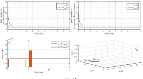
The results can be seen on Fig. 5. The upper left diagram shows the change of the state variables of the reference LTI systemS(p_{re f})over time, while the upper right diagram represents the simulation results over time of the state variables of the parameter dependent LPV systemS(p(t)). The difference (error) between them is represented by the lower left diagram. However, as thep(t)varies over time (as the lower right diagram shows), there is only numerical difference between the states of S(p_{re f})andS(p(t)). That means, the LPV system and indirectly, the original nonlinear system, precisely mimics the behavior of the reference LTI system over time. Since, the given example is a physiological one, we tried the accuracy of the proposed controller structure, if there is a saturation on the control input, which

Time [min]

0 1 2 3 4 5 6 7 8 9 10

State variables of the reference system

5 10 15 20 25 30

x_1,ref(t) x2,ref(t)

Time [min]

0 1 2 3 4 5 6 7 8 9 10

State variables of the parameter dependent system ₅ 10 15 20 25 30

x_1,par(t) x2,par(t)

Time [min]

0 5 10 15

State errors

×10^-15

-1 -0.5 0 0.5 1 1.5 2

x1,ref(t)-x 1,par(t) x_2,ref(t)-x_2,par(t)

0.6 0.7 p_ref

0.4 0.5

p₁(t) 0.2 0.3 0 0.1 ppar,end

5 p₂(t) p_par,start

10 0.4 0.2 0 0.8 0.6

15 p3(t)

Figure 5

Results of the simulation without control input saturations

does not allow the occurrence of physiological not relevant control inputs (control inputs only can be positive or has to be higher than a given amount). We have found that the results are different than the previous case, which mostly come from that fact, that the selected scheduling variables are dependent from the actual values of the states. Namely, the state variables are coupled to theS(p(t))through thep(t).

However, we did not use any saturation on the values of the state variables to com- pensate the effect of the saturation.

Figure 6 represents this latter scenario, when saturation is applied. Each parame- ter turned to be the same during the simulation, except that we consider that the input signal cannot be negative at all. The results shows that there is a difference between the states ofS(p_{re f})andS(p(t))over time. However, the controller can handle the situation and can provide stable control for S(p(t)). The difference is slowly decreasing and the state variables reach the predefined reference levels.

Conclusions

In this paper we introduced a novel LPV-based controller design approach. This method provides a mixture of classical, optimal state-feedback control and a sup- plementary control, which is based on the 2-norm difference between parameter vectors (and belonging parameter dependent LTI systems) of the LPV parameter space. The main advantage of the proposed controller structure is that it is sufficient to design a reference controller for a reference LTI system and the actual, neces- sary control action, over time, will be determined by comparison to this reference controller through algebraic manipulations. Moreover, the LPV system will mimic the behavior of the reference system over time, requiring an appropriately selected reference LTI system. The completed controller can thus guarantee the stability of the system. Moreover, it is enough to determine performance specifications only for the reference LTI system - due to the completed controller forces, the LPV system will aquire these specifications, as well.

Time [min]

0 1 2 3 4 5 6 7 8 9 10

State variables of the reference system

5 10 15 20 25 30

x_1,ref(t) x2,ref(t)

Time [min]

0 1 2 3 4 5 6 7 8 9 10

State variables of the parameter dependent system ₅ 10 15 20 25 30

x_1,par(t) x2,par(t)

Time [min]

0 5 10 15

State errors

-8 -6 -4 -2 0 2

x1,ref(t)-x 1,par(t) x2,ref(t)-x

2,par(t) 0.6 0.7

p_ref

0.4 0.5

p₁(t) 0.2 0.3 0 0.1 ppar,end

5 p₂(t) p_par,start

10 0.8 0.6 0.4 0.2 0 15 p3(t)

Figure 6

Results of the simulation with control input saturations

Acknowledgement

Gy. Eigner thankfully acknowledge the support of the Robotics Special College of ´Obuda University. The research was supported by the Research and Innovation Center of ´Obuda University.

References

[1] W. S. Levine. The Control Engineering Handbook. CRC Press, Taylor and Francis Group, Boca Raton, 2nd edition, 2011.

[2] J. K. Tar, J. F. Bit´o, L. N´adai, and J. A. T. Machado. Robust Fixed Point Transformations in Adaptive Control Using Local Basin of Attraction. ACTA Polytechnica Hungarica, 6(1):21–37, 2009.

[3] A. P. White, G. Zhu, and J. Choi.Linear Parameter Varying Control for Engi- neering Applicaitons. Springer, London, 1st edition, 2013.

[4] P. Baranyi, Y. Yam, and P. Varlaki. Tensor Product Model Transformation in Polytopic Model-Based Control. Series: Automation and Control Engineering.

CRC Press, Boca Raton, USA, 1st edition, 2013.

[5] R. S. Burns, editor. Advanced Control Engineering. Butterworth-Heinemann, Oxford, UK, 1st edition, 2001.

[6] D. J. Leith and W. E. Leithead. Survey of gain-scheduling analysis design.

International Journal of Control, 73:1001–1025, 1999.

[7] D.W. Gu, P.H. Petkov, and M.M. Konstantinov. Robust Control Design with Matlab. Springer, London, UK, 2nd edition, 2013.

[8] W. S. Levine, editor.The Control Engineering Handbook. CRC Press, Taylor and Francis Group, Boca Raton, USA, 2 edition, 2011.

[9] O. Sename, P. G´asp´ar, and J. Bokor. Robust control and linear parameter varying approaches, application to vehicle dynamics. volume 437 ofLecture Notes in Control and Information Sciences. Springer-Verlag, Berlin, 2013.

[10] L. Kov´acs, B. Beny´o, J. Bokor, and Z. Beny´o. Inducedl2-norm minimization of glucose–insulin system for type I diabetic patients. Comput. Meth. Prog.

Bio., 102(2):105 – 118, 2011.

[11] Gy. Eigner, J. K. Tar, I. Rudas, and L. Kov´acs. LPV-based quality interpre- tations on modeling and control of diabetes. ACTA Polytechnica Hungarica, 13(1):171 – 190, 2016.

[12] J. Kuti, P. Galambos, and P. Baranyi. Minimal volume simplex (mvs) convex hull generation and manipulation methodology for tp model transformation.

Asian Journal of Control, 2015. submitted.

[13] F. Wettl. Linear Algebra [in Hungarian]. Budapest University of Technology and Economy, Faculty of Natural Sciences, Budapest, Hungary, 1nd edition, 2011.

[14] R. A. Beezer.A First Course in Linear Algebra. Congruent Press, Washington, USA, version 3.40 edition, 2014.

[15] J. K. Tar, L. N´adai, I. Felde, and I. J. Rudas. Advances in Robot Design and Intelligent Control: Proceedings of the 24th International Conference on Robotics in Alpe-Adria-Danube Region (RAAD), chapter Cost Function-Free Optimization in Inverse Kinematics of Open Kinematic Chains, pages 137–

145. Springer International Publishing, 2016.

[16] J. D. Bronzino and D. R. Peterson, editors.The Biomedical Engineering Hand- book. CRC Press, Boca Raton, USA, 4th edition, 2016.