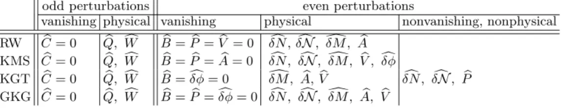
Gravitational dynamics in a 2+1+1 decomposed spacetime along nonorthogonal double foliations: Hamiltonian evolution and gauge fixing

(1)

arXiv:1905.00039v1 [gr-qc] 30 Apr 2019

Gravitational dynamics in a 2+1+1 decomposed spacetime along nonorthogonal double foliations: Hamiltonian evolution and gauge fixing

Cec´ılia Gergely, Zoltán Keresztes, and László Á. Gergely Institute of Physics, University of Szeged, Dóm tér 9, 6720 Szeged, Hungary

(Dated: May 2, 2019)

Motivated by situations with temporal evolution and spatial symmetries both singled out, we develop a new 2+1+1 decomposition of spacetime, based on a nonorthogonal double foliation. Time evolution proceeds along the leaves of the spatial foliation. We identify the gravitational variables in the velocity phase-space as the 2-metric (induced on the intersection Σtχof the hypersurfaces of the foliations), the 2+1 components of the spatial shift vector, together with the extrinsic curvature, normal fundamental form and normal fundamental scalar of Σtχ, all constructed with the normal to the temporal foliation. This work generalizes a previous decomposition based on orthogonal foliations, a formalism lacking one metric variable, now reintroduced. The new metric variable is related to (i) the angle of a Lorentz-rotation between the nonorthogonal bases adapted to the foliations, and (ii) to the vorticity of these basis vectors. As a first application of the formalism, we work out the Hamiltonian dynamics of general relativity in terms of the variables identified as canonical, generalizing previous work. As a second application we present the unambiguous gauge- fixing suitable to discuss the even sector scalar-type perturbations of spherically symmetric and static spacetimes in generic scalar-tensor gravitational theories, which has been obstructed in the formalism of orthogonal double foliation.

I. INTRODUCTION

The modern theory of gravitation, general relativity (GR) has been successfully tested multiple times on the Solar Sytem scale. When confronted with observations on both galactic scales and beyond, agreement with pre- dictions can however be reached only at the price of introducing dark matter and dark energy, neither of them identified or detected by other means than gravitational.

Lacking indications on manifestations of these forms of matter in the Standard Model interactions, they could be included in the gravitational sector, either as geometric modifications arising from possible higher-order dynamics or as an excess of fields representing gravity beyond the metric tensor, possibly including scalars, vectors, 2- form fields or even a second metric. As a rule, the physical metric couples to these in a nonminimal way, opposed to dark matter/dark energy models, which are coupled minimally. The simplest such model, of a single scalar field complementing the metric has been studied exten- sively, both from the desire to explain dark matter / dark energy or in order to study inflation.

The most generic single scalar-tensor model described by second order differential equations (hence avoiding Os- trogradski instabilities) for both the metric and the scalar field has been proposed by Horndeski [1] and rediscov- ered in a modern context in connection with generalized galileons [2].

While allowing for higher order than two, certain beyond Horndeski models could guarantee that the propa- gating degrees of freedom (d.o.f.) still evolve according to a second order dynamics. Indeed, an effective field theory (EFT) of cosmological perturbations has been worked out by Gleyzes et al. [3, 4], based on (a) a Lagrangian depending on the lapse function and some geometrical scalar quantities emerging in the Arnowitt-Deser-Misner

(ADM) decomposition on the flat Friedmann-Lemaˆıtre- Robertson-Walker (FLRW) background and (b) the uni- tary gauge, allowing to absorb the scalar field perturbation by an adequate time coordinate choice (the lapse is then associated with the corresponding constant scalar- field hypersurfaces). The linear perturbation equations contain time derivatives at second order, although spatial derivatives could be of higher order (in the Horndeski subclass the latter are also of second order). A generalization for two scalar fields representing dark matter and dark energy has been advanced in Ref. [5]. Another generalization has been discussed in Ref. [6], referring to perturbations of a spherically symmetric and static background, treated similarly.

These theories should obey the requirements of (A) stability, guaranteed by the avoidance of both

scalar ghosts (no negative kinetic term in the second order Lagrangian governing the evolution of linear perturbations) and Laplacian instabilities (no negative sound speed squared),

(B) agreement with Solar System tests, notably the Vainshtein mechanism suppressing the propagation of the fifth force inside the Solar System (no L5

contribution to the Horndeski Lagrangian) [7–9], (C) agreement with weak lensing observations (con-

straints from deviations from the Newtonian law and light bending by simultaneous fitting of x-ray and lensing profiles of galaxy clusters) [10].

The recent detections of gravitational waves from 10 coalescing binary black holes and one neutron star merger by the LIGO Scientific Collaboration and Virgo Collab- oration [11–17] have added new constraints. On the one hand, the mass of the graviton has been severely constrained by testing a massive dispersion relation [18].

(2)

Then a wide family of dispersion relations [19] were tested, disruling [13] Lorentz-violation, Hoˇrava-Lifsic theories, certain extra dimensional, multifractal theories, doubly special relativity and setting an even harder constraint on the graviton mass at 5.0×10⁻²³eV/c²[20]. On the other hand the small difference in the arrival time of the gravitational waves from a neutron star coalescence [16] and accompanying γ−radiation confirmed that the tensorial gravitational modes propagate with the speed of light within−3×10⁻¹⁵and +7×10⁻¹⁶accuracy [21].

By exploring previously existing analyses on the Lapla- cian stability and ghost avoidance in Horndeski theories [22, 23], from these constraints the L5 contribution has been disruled once again, together with the kinetic term dependence ofL4[24–26]. A slightly less restrictive con- dition emerged for the beyond Horndeski models. Fur- ther, three of the five parameters appearing in the effective theory of dark energy were severely constrained by combining the gravity wave results with galaxy cluster observations [27].

The stability of spherically symmetric, static spacetimes has been discussed for both the odd [28] and even modes [29] of the perturbations in Horndeski theories, also for the odd modes in the beyond Horndeski theories [6]. The latter relied on a double foliation of spacetime along orthogonal spatial and temporal leaves, developed in Refs. [30, 31]. Three independent background dynamical equations were identified and the conditions for avoidance of ghosts and Laplacian instabilities of the odd mode perturbations established.

The formalism of the orthogonal double foliation relies on the extensive use of adapted metric variables, which bear the role of canonical coordinates and on embedding variables (extrinsic curvatures, normal fundamental forms and normal fundamental scalars of the 2-surfaces generated by the intersection of the foliations), some of them emerging as canonical momenta, others as pure spatial derivatives of the coordinates. The odd sector of perturbations of spherically symmetric, static spacetimes has been analyzed in terms of these quantities [6].

Spacetime perturbations can also be discussed through other decomposition techniques, including: (I) the first order system of 70 coupled differential equations for 50 independent variables of the black hole perturbation formalism `a la Chandrasekhar [32], based on the Newman- Penrose formalism (an 1+1+1+1 decomposition); (II) the formalism based on the numerous variables arising from a 2+1+1 decomposition based on kinematical quantities (optical scalars), supplemented by the electric and magnetic projection of the Weyl tensor [33, 34]; (III) a (2+1)+1 decomposition based on the introduction of the quotient space defined by the orbits of a rotational Killing vector [35, 36]; (IV) a temporal foliation followed by a further 2+1 slicing to deal with axisymmetric and sta- tionary configurations [37], generalized later on for a 2+1 foliation of a hypersurface with arbitrary causal character [38, 39], a technique also employed in Ref. [40] for identifying a hyperbolic system in the constraint struc-

ture, rewritten in terms of the 2+1 decomposition of the extrinsic curvature of the hypersurfaces explored previously in the orthogonal double foliation formalism of Ref.

[30]; (V) the standard metric perturbation formalism, explored in a spherically symmetric, static setup in Refs.

[28, 29]. The advantage of the orthogonal double foliation formalism over the first two consist in its substantially reduced number of variables. A comparison with the third and fourth has been presented in [30]. The third relies heavily on the use of a Killing vector, which is not a necessity for the orthogonal double foliation. Although the fourth approach contains the same number of metric variables (9), it does not employ all geometric quantities playing an essential role in Refs. [30, 31]. In particular, Ref. [38] introduces a second fundamental form combining a set of dynamical and nondynamical variables explored in Refs. [30, 31], a normal fundamental form but no normal fundamental scalar. Finally, the advantage over the metric perturbation formalism is the canonical (geometrodynamical) interpretation of the variables.¹

The simplicity of the orthogonal double foliation of Refs. [30, 31] however required to waste one gauge d.o.f.

for imposing the orthogonality requirement after the perturbation. This hampered the discussion of the even modes, carrying an arbitrary function of time, hence los- ing their physical interpretation [6].

It is the purpose of the present paper to lift the condi- tion of orthogonality of the two foliations in order to recover the full power of gauge fixing and open the way for the discussion of the even mode perturbations in generic scalar-tensor theories on a spherically symmetric, static background, complementing the similar discussion of the odd sector.

The paper is organized as follows. In Sec. II we develop the new 2+1+1 decomposition of the spacetimeB based on two nonorthogonal foliations, one of them temporal (S^t, characterized by constant t), the other one spatial (M_χ, with constantχ). This generalizes the formalism of the orthogonal double foliation of spacetime, developed in Refs. [30, 31], by allowing for a 10th metric functionN. We adapt suitable bases to both foliations, then give the evolutions along the ∂/∂tand ∂/∂χ con-

1Other spacetime decomposition techniques are also known. Ap- plying the formalism developed in the seminal monograph [41], a 2+2 breakup of the field equations was advanced in Ref. [42]

with the aim of identifying the gravitational d.o.f. in the so-called conformal two-structure (the latter representing the information on how the family of selected 2-surfaces is embedded in a 3- surface). For the discussion of the initial value problem Ref. [43]

developed the 2+2 decomposition of spacetime in detail, based on space-like 2-surfaces{S}rigged by a dyad basis given by their two mutually orthogonal normals (and the respective orthogonal 3-foliations). Then the covariant derivatives of these normals were decomposed in terms of the extrinsic curvatures of {S}, the induced connection of the timelike 2-surface{T}spanned by the dyad basis and the curvature tensor of {T}. The Einstein equations were decomposed accordingly.

(3)

gruences (tangent to M_χ and St, respectively) in both bases. Two of the basis vectors (tangent to the intersection Σtχ of S^t and M_χ) are common in both bases, while the other two pairs are related by a Lorentz rotation with angleφ= tanh⁻¹(N/N), whereN is the lapse function. Another geometric interpretation of the 10th metric function arises as the vorticity of the basis vectors orthogonal to both the hypersurface normals (of the same basis) and to Σtχ. This is shown here through the discussion of the algebras of each basis vectors and in the discussion of the vorticities in the two Appendices.

In Sec. III we characterize the embedding in terms of extrinsic curvatures, normal fundamental forms and normal fundamental scalars of the hypersurface normals, also introduce the 2+1 decomposed form of the curvature of their congruences (their nongravitational accelerations). For the basis vectors orthogonal to them we introduce similar quantities. We establish the intercon- nections among all those geometric quantities. In Sec.

IV we also derive their connection with the time- and χ-derivatives of the metric functions. This enables us to select those geometric variables, which bear a dynamical role, e.g., connected to canonical momenta.

As a first application, we present the Hamiltonian formalism of general relativity in the 2+1+1 decomposed form in Sec. V. We derive the canonical momenta, then the Hamiltonian and diffeomorphism constraints and the boundary terms of the action, all in terms of canonical data defined on Σtχ. We recover previous results of Ref.

[31] applying for the orthogonal double foliation in the vanishing N limit. The nonorthogonality of the foliations also generates new terms.

Then, in Sec. VI we explore the diffeomorphism gauge freedom for fixing the perturbations on the static and spherically symmetric background of beyond Horndeski theories in an unambiguous way. This result opens up the possibility for the discussion of the even sector of the perturbations. Although the unambiguous gauge fixing is different from the one employed for the odd sector in Ref. [6], the results of the stability analysis presented there are unaffected, as the two sectors decouple.

In Sec. VII we present our conclusions. Two Appen- dices are devoted to discuss the consequences of the hypersurface orthogonality of the normal basis vectors and the interpretation of the vorticities of the complemen- tary basis vectors in terms of the geometric quantities introduced in the main body of the paper.

We use the abstract index notation throughout the paper. Latin and greek indices, respectively, denote 4-dimensional spacetime and 3-dimensional spatial abstract indices. Boldface lower- and uppercase indices dif- ferentiate among 2-dimensional and 4-dimensional basis vectors, respectively. 4-dimensional quantities will carry a distinguishing tilde sign, while 3-dimensional quantities a overhat (or reversed overhat) sign. Tensors defined both on the full spacetime and on lower-dimensional (hy- per)surfaces carry Latin indices, the latter obeying the required projection conditions. Quantities defined on the

background in a perturbational setup carry an overbar.

Round or square brackets on indices denote symmetriza- tion or antisymmetrization, respectively.

II. THE NONORTHOGONAL 2+1+1 DECOMPOSITION OF SPACETIME LetBbe a 4-dimensional manifold with metric ˜gab of Lorentzian signature. We assume the manifold admits both a timelike and a spacelike foliation. In this section we generalize the formalism of [30, 31] by dropping the orthogonality requirement of the foliationsS^t(with constant time coordinate t) and M_χ (with constant space coordinateχ).

On the tangent space of the doubly-foliable spacetime B we introduce the bases eA = {∂/∂t, ∂/∂χ, Ei} (with Eisome basis elements of the tangent space of Σtχ) and its dual e^B =

dt, dχ, E^j on the respective cotangent space.

Letnâ be the (timelike) unit normal to St, while mâ the (spacelike) unit normal to both nâ and Σtχ. With them we introduce the basis fA = {n, m, Fi} adapted to S^t (with Fi basis elements of the tangent space of Σtχ) and its dualf^B=

¯

n,m, F¯ ^j . The (spacelike) unit normal toM_χ islâ, whilekâ denotes the (timelike) unit normal to both lâ and Σtχ. The basis adapted to M_χ is gA = {k, l, Gi} (where Gi are basis elements of the tangent space of Σtχ), withg^B=¯k,¯l, G^j its dual.

For simplicity one can chose coordinate basis vectors Ei=Fi=Gi=∂/∂yⁱ. From the causal character of the basis vectors and from the duality relations we get

¯

na = −na , m¯a =ma , k¯a = −ka , ¯la=la .

A. The induced metric

The 4-metric ˜gabcan be decomposed in two equivalent ways

˜

gab = −nanb+mamb+gab, (1)

˜

gab = −kakb+lalb+gab . (2) As usual ˜g^b_a ≡δ_a^b, while the mixed form of the induced metricgab projects to Σtχ. With this projection, both covariant derivatives and Lie derivatives along a congruence V^a of any 4-dimensional tensor ˜T_b^a¹^...a^r

1...br could be projected onto Σtχ:

DaT˜_b^a¹^...a^r

1...bq ≡g^c_ag^a_c₁¹...g_c^a_r^rg_b^d¹

1...g^d_b^q

q

∇˜^cT˜_d^c¹^...c^r

1...dq , (3) L_VT˜_b^a¹^...a^r

1...bq ≡g_c^a¹

1...g^a_c_r^rg_b^d¹

1...g_b^d^q

q

˜

L_VT˜_d^c¹^...c^r

1...dq . (4) We note that whenever ˜T_b^a¹^...a^r

1...bq is a projected object onto Σtχ, the expression DaT˜_b^a¹^...a^r

1...bq is exactly the covariant derivative in Σtχ (which annihilates gab), while

(4)

L_VT˜_b^a¹^...a^r

1...bq describes an evolution along the congruence V^a (it represents the partial derivative with respect to the adapted coordinatev, thusV=∂/∂v, wherevcould be eithertorχ). Otherwise they become but notations, as they fail to obey the Leibniz rule [30]).

B. Evolutions in the fA basis

The first two elements of the coordinate basis eA, representing evolution vectors can be generically decomposed in thefAbasis as

∂

∂t a

= N nâ+Nâ+Nmâ , (5) ∂

∂χ a

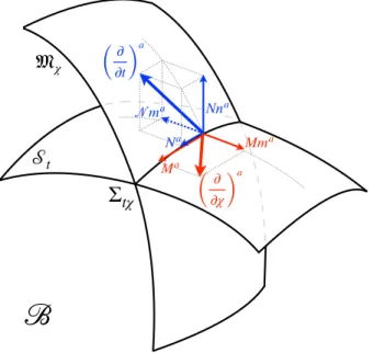
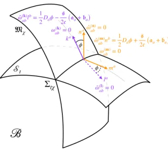
= M mâ+Mâ+Mnâ . (6) Here Nâ and Mâ (N and M) are the components of the 3-dimensional shift vectors along (orthogonal to) Σtχ, whileN andM represent lapse type functions of the respective evolutions. Together with the 3 independent components ofgabthere seem to be 11 gravitational variables at this stage, but their number will be reduced to 10. Indeed, the duality relation hdt, ∂/∂χi= 0 implies M= 0, which in turn implies through Eq. (6) that∂/∂χ is tangent toS^t, see also Fig. 1.

𝔐χ

𝒮

_t

Σ

_t

χ

ℬ

(

∂

∂t)

a

(

∂

∂χ) M^a a

Nn^a

Mm^a N^a

𝒩m^a

FIG. 1: The decomposition of the temporal and radial evolution vectors in thefA basis. (For visualization purposes a negativeN was chosen.)

From the rest of the duality relations e^B, eA

= δ^B_A one gets

¯

n = N dt ,

¯

m = Ndt+M dχ ,

F^j = N^jdt+M^jdχ+E^j . (7)

As∂/∂tis timelike andN^a spacelike, the inequalities N²− N²> gabN^aN^b≥0

hold, while ∂/∂t lying in the future light cone implies N >0.

We conclude this subsection by giving in Table I the algebra of the basis vectorsfA. As expected from the Frobenius theorem, the basis vectors {m, Fi} span the tangent space of S^t, while from the dual form of the Frobenius theorem the fourth basis vectornâ turns out vorticity-free (also shown explicitly in Appendix A). The same type of reasoning yields that mâ has vorticity (as the component along mâ of the [n, Fj] bracket is nonvanishing, hence the vectors {n, Fi} do not span a hypersurface). This vorticity is given in Appendix B and disappears together with N in the orthogonal foliation limit employed in Refs. [30, 31]. Hence the vorticity of the basis vectormâis generated by the nonorthogonality of the two foliations.

C. The role of the 10th metric variable

The new element in the formalism as compared with that of Refs. [30, 31] is the shift componentN, which reestablishes the number of gravitational variables as 10, equivalent to the 4-metric variables.

Straightforward calculations employing also the rest of the duality relations

f^B, fA

=δ_A^B= g^B, gA

and Eqs.

(7) lead to the relation between the two adapted bases ¯k

¯l

=

c −s

−s c

¯ n

¯ m

, (wheres= sinhφ,c= coshφ) and

k^a l^a

= c s

s c n^a m^a

, (8)

thus in the form of a Lorentz-rotation. Its angle is defined by

N =Ntanhφ . (9) This represents the second geometric interpretation of the 10th metric variable (beyond the vorticity ofm).

D. Evolutions in thegA basis

With the Lorentz rotations given in the previous subsection it is easy to express the evolution vectors in the gAbasis:

∂

∂t a

= N

ck^a+N^a , (10) ∂

∂χ a

= M(−skâ+clâ) +Mâ . (11)

(5)

[n, m]â [n, Fj]â [m, Fj]â nâ _M¹

∂χ(lnN)−_M¹M^j∂j(lnN)

∂j(lnN) 0 m^a _{M N}¹

−∂tM+∂χN+N^j∂jM−M^j∂jN _M

N∂j N M

∂j(lnM) F_i^a _{M N}¹ −∂tMⁱ+∂χNⁱ+N^j∂jMⁱ−M^j∂jNⁱ ₁

N

∂jNⁱ−_M^N∂jMⁱ ∂_jMⁱ M

TABLE I: The algebra of the basis vectorsfA. The components of the brackets enlisted in the first line along the vectors in the first column are given.

𝔐χ

𝒮

_t

Σ

_t

χ

ℬ

(

∂

∂t)

a

N

𝔠 k^a

𝔠Ml^a

−𝔰Mk^a

N^a

M^a

(

∂

∂χ)

a

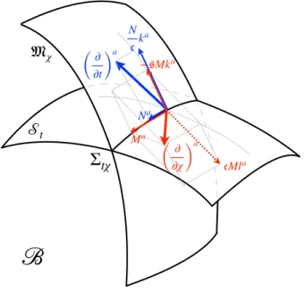
FIG. 2: The decomposition of the temporal and radial evolution vectors in thegAbasis. (For visualization purposes a negativeswas chosen.)

Remarkably, the evolution vector∂/∂thas no component alongl, hence it is tangent toM_χ, see also Fig. 2.

Further exploring the duality relations one gets

¯k = −Msdχ+N c dt ,

¯l = Mcdχ ,

G^j = N^jdt+M^jdχ+E^j=F^j . (12) The algebra of the basis vectorsgAis presented in Table II. Again, from the Frobenius theorem, the basis vectors {k, Gi}span the tangent space ofM_χ and from its dual form the fourth basis vector l^a turns out vorticityfree.

The vectork^a however has vorticity (as the component alongk^a of the [l, Gj] bracket is nonvanishing). This vorticity is given in Appendix B and again disappears with N in the orthogonal foliation limit employed in Refs.

[30, 31]. Hence the vorticity of the basis vector k^a is also generated by the nonorthogonality of the two foliations. Finally we note that in the orthogonal foliation limit N → 0 the algebras given in Tables I-II coincide and the vorticities of the basis vectors disappear.

III. CODIMENSION-2 EMBEDDING OF Σtχ

In this section we introduce a series of geometrical quantities characterizing the embedding of Σtχ and we analyze their relationship with various coordinate derivatives of the metric variables.

We have defined a total of four normals to the surface Σtχ, two pairs taken from the bases fA and gA, respectively. With each of them we define an extrinsic curvature, as follows:

Kab ≡ Danb= 1 2L_ngab , Lab ≡ Dalb=1

2L_lgab , K_ab^∗ ≡ Dakb= 1

2L_kgab, L^∗_ab ≡ Damb= 1

2L_mgab . (13) All these tensors are symmetric, as shown in the Appen- dices A and B.

With the two normals to the hypersurfaces we define the normal fundamental forms of Σtχ as follows:

K^a ≡ g_a^cm^d∇˜^cnd=g^c_am^d∇˜^dnc,

La ≡ −g^c_ak^d∇˜cld=−g^c_ak^d∇˜dlc . (14) Their second expressions arise from the hypersurface- orthogonality of the basis vectorsn^a and l^a, as proven in Appendix A. It is easy to prove that they are related as

Lâ=Kâ+Daφ . (15) By contrast, for the vectors kâ and mâ (which have vorticity) the similarly defined quantities

K^∗a ≡ g^d_al^c∇˜^ckd ,

L^∗a ≡ −g_a^dn^c∇˜cmd (16) do not share this interchangeability property. Similarly, one can prove

L^∗a=K^∗a+Daφ . (17) The differences K^∗a− La and L^∗a − Ka give the nonvanishing components of the vorticities of k^a and m^a, respectively, as demonstrated in Appendix B.

(6)

[k, l]â [k, Gj]â [l, Gj]â kâ

∂t s N

−N^j∂j s N

+_N^s

∂tln (M N)−N^j∂jln (M N)

∂j ln^N_c

−_c2^NM∂j scM N

+_cM¹

∂χln ^N_c

−M^j∂jln ^N_c

l^a _{M N}¹

−∂t(cM) +N^j∂j(cM)

0 ∂jln (cM) G^a_i _{M N}¹

−∂tMⁱ+∂χNⁱ−M^j∂jNⁱ+N^j∂jMⁱ c

N ∂jNⁱ s

N∂jNⁱ+_cM¹ ∂jMⁱ

TABLE II: The algebra of the basis vectorsgA. The components of the brackets enlisted in the first line along the vectors in the first column are given.

For the hypersurface-orthogonal vectorsn^aandl^anor- mal fundamental scalars

K ≡ m^dm^c∇˜^cnd,

L ≡ k^dk^c∇˜cld (18) can be defined. The corresponding quantities for the basis vectorsk^a andm^a are

K^∗ ≡ l^dl^c∇˜^ckd ,

L^∗ ≡ n^cn^d∇˜cmd . (19) Finally the two timelike vector congruences have the curvatures (nongravitational 3-dimensional accelerations):

ˆ

αa ≡n^b∇˜^bna=a_a−maL^∗ , (20) ˆ

α^∗_a ≡k^b∇˜^bka=a^∗

a−laL, (21)

the second set of expressions representing their 2+1 decomposed form with the 2-dimensional acceleration components:

a_a ≡ g_a^cn^b∇˜bnc , a^∗

a ≡ g_a^ck^b∇˜^bkc . (22) Similarly, the spacelike congruencesl^a andm^a have the 3-dimensional curvatures:

βˇa ≡l^b∇˜bla=b_a+kaK^∗ , (23) βˇ_a^∗≡m^b∇˜^bma=b^∗

a+naK , (24)

with the 2-dimensional “acceleration” components:

b_a ≡ g_a^dl^c∇˜cld , b^∗

a ≡ g_a^dm^c∇˜^cmd . (25) With the above-introduced quantities the 2+1+1 decomposition of the covariant derivatives of the normals to Σtχ in the bases they belong is

∇˜^anb = Kab+ 2m(aK^b)+mambK+nambL^∗

−naa_b , (26)

∇˜^alb = Lab+ 2k(aL^b)+kakbL+lakbK^∗

+lab_b , (27)

∇˜^akb = K_ab^∗ +laK^∗b+lbL^a+lalbK^∗+kalbL

−kaa^∗_b , (28)

∇˜^amb = L^∗_ab+naL^∗b +nbK^a+nanbL^∗+manbK +mab^∗

b . (29)

For deriving Eqs. (26), (27) we have also employed the second equalities (14). The structure of Eqs. (28), (29) is slightly different due to the vorticities of the vectors k^a andl^a.

The geometric quantities defined in this subsection are not all independent. This should be obvious as the two bases are related by a Lorentz-rotation. By tedious but straightforward algebra we expressed all starry quantities in terms of unstarred ones and φ (or N). For example the extrinsic curvatures defined with the basis vectors of the two bases are related by a rotation matrix with angle ψ= arccos (1/coshφ) as:

K_ab^∗ L^∗_ab

=

1/c s/c

−s/c 1/c

Kab

Lab

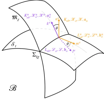
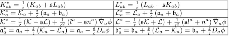
. (30) The geometric quantities characterizing the embedding are summarized on Fig. 3 while the full set of interde- pendencies are given them in Table III.

𝔐χ

𝒮

_t

Σ

_t

χ

ℬ

n^a

lâ mâ kâ

ϕ

K_ab,𝒦_a,𝒦,𝔞_a K*_ab,𝒦*_a,𝒦*,𝔞*_a

L_ab,ℒ_a,ℒ,𝔟_a

L_ab*,ℒ*_a,ℒ*,𝔟*_a

FIG. 3: The geometric embedding variables.

Note that the notations were introduced such that in the particular caseN = 0 all starry quantities transform into the corresponding unstarred ones (e.g.,K_ab^∗ becomes Kab). Further, as in that case the vorticities of the basis vectorskâ andmâ vanish,Lâ=Kâ (as explored in Refs.

[30, 31]) follows.

(7)

K_ab^∗ = ¹_c(Kab+sLab) L^∗_ab=¹_c(Lab−sKab) K^∗a=Ka+^s_c(a_a+b_a) L^∗a=La+^s_c(a_a+b_a)

K^∗=¹_c(K −sL) +_c¹2(lâ−snâ) ˜∇aφ L^∗=¹_c(sK+L) +_c¹2(slâ+nâ) ˜∇aφ a^∗_a=a_a+^s_c(Ka− La) =a_a−^s_cDaφ b^∗_a=b_a+^s_c(La− Ka) =b_a+^s_cDaφ

TABLE III: The relations among starred and unstarred geometric quantities characterizing the embedding of Σtχ.

IV. KINEMATICS AND GEOMETRIC EMBEDDING

In this section we establish the relations of the temporal and spatial derivatives of the metric variables {gab, M^a, M} to the geometric quantities K^ab, Ka, K ,

L^ab, La, L ,

K^∗^ab, K^∗a, K^∗ and L^∗^ab, L^∗a, L^∗ characterizing the embedding. These will be used later in the derivation of the Hamiltonian formulation of GR from the Einstein-Hilbert action.

Bearing in mind that both the coordinate derivatives along time and χ and the extrinsic curvatures are projected Lie derivatives, we find for the extrinsic curvature in the two bases

Kab = 1 N

1

2∂tgab−D(aNb)

− s Mc

1

2∂χgab−D(aMb)

, L^∗_ab = 1

M 1

2∂χgab−D(aMb)

(31) and

Lab = s N

1

2∂tgab−D(aNb)

+ 1

Mc 1

2∂χgab−D(aMb)

, K_ab^∗ = c

N 1

2∂tgab−D(aNb)

, (32)

respectively. OnlyL^∗_abis free from time derivatives of the induced metric, hence nondynamical.

In order to establish the relation of the rest of the geometric variables with time and χ-derivatives of the metric variables we employ the following identity holding for all vectorsVI for which ˜g(VI, VJ) =constant:

˜

g(VA,∇˜^VBVC) = ˜g([VA, VB], VC)

−g(V˜ C,∇˜VAVB). (33) First we apply this identity for the case VB = VC, such that the last term vanishes. Then for the basis vectors fA and gA perpendicular to Σtχ the left- hand sides are the accelerations ˆαa = ˜g

fA,∇˜ⁿn f_a^A, ˆ

α^∗_a = ˜g

gA,∇˜^kk

g^A_a, ˇβa = ˜g

gA,∇˜^ll

g_a^A and ˇβ_a^∗ =

˜ g

fA,∇˜^mm

f_a^A. Calculating the right-hand sides by exploring the specific components of the Lie brackets given in Tables I and II and comparing the resulting expressions with the decompositions given in Eqs. (20),

(21), (23) and (24) we obtain the 2-dimensional accelerations as projected covariant derivatives

a_a = Da(lnN) , b^∗

a = −Da(lnM) , b_a = −Daln (cM) , a^∗

a = Da

lnN

c

, (34)

while the normal fundamental scalars emerge as K = 1

M N [∂tM −∂χN −N^aDaM+M^aDaN] , L^∗ = − 1

M [∂χ(lnN)−M^aDa(lnN)] , L = −S − 1

cM

∂χln N

c

−M^aDaln N

c

, K^∗ = 1

M N [∂t(cM)−N^aDa(cM)] , (35) with

S = ∂t

s N

−N^aDa

s N

+s

N [∂tln (M N)−N^aDaln (M N)] (36) (an expression which vanishes for orthogonal foliations).

Next we apply the identity (33) for n^b∇˜bma =

˜ g

fA,∇˜ⁿm

f_a^A and l^b∇˜^bka = ˜g

gA,∇˜^lk

g_a^A, respectively, obtaining for the Σtχ projections

L^∗a = K^a+M NDa

N M

, (37)

K^∗a = L^a− N c²MDa

scM N

. (38)

These can be also derived from the expressions given in Table III together with Eqs. (15) and (34). Now we have everything at hand to derive the relation of the normal fundamental forms and metric derivatives. For this we rewrite

K^a = −gab[m, n]^b− L^∗a , La = −gab[k, l]^b− K^∗a ,

employ the algebras of the basis vectorsfA andgAgiven in Tables I and II, respectively, together with Eqs. (37)

(8)

and (38), to obtain K^a = 1

2M N ∂tMâ−∂χNâ−N^bDbMâ+M^bDbNâ

−M 2ND^a

N M

, L^a = 1

+ N

2c²MD^a scM

N

, K^∗^a = 1

− N 2c²MD^a

scM N

, L^∗^a = 1

2M N ∂tMâ−∂χNâ−N^bDbMâ+M^bDbNâ +M

2ND^a N

M

. (39)

Note that the metric derivatives are related to the normal fundamental vectors, rather then forms.

From the results of this and of the previous section we can conclude that the independent metric variables with dynamical role are{gab, M^a, M}while the embedding variables

K^ab, K^a, K carry information about their temporal evolution. The extrinsic curvatureL^∗_abbe- ing the only one, which contains no time derivatives, it plays a nondynamical role. Hence we chose the variables emerging in thefAbasis as independent,

K^ab, K^a, K representing momenta, while

L^∗^ab, L^∗ merely spatial derivatives. All other embedding variables can be expressed in terms of this set.

V. HAMILTONIAN FORMALISM IN GENERAL RELATIVITY

In this section we present the 2+1+1 decomposed Hamiltonian formalism in general relativity. As discussed earlier, we employ thefA basis in the decomposition.

A. The 2+1+1 decomposition of the Einstein-Hilbert action

We define the 2-dimensional Riemann tensorRabcd of the metric induced in Σtχ as

RabcdV^b= (DcDd−DdDc)Va , (40) which written in terms of the geometric quantities arising in the 2+1+1 decomposition and of the 4-dimensional Riemann tensor leads to the following Gauss-type identity:

Rabcd=g_aⁱg_b^jg_c^kg_d^lR˜ijkl+ 2

L^∗_a[cL^∗_d]b−Ka[cKd]b

. (41)

The extrinsic curvatures are those appearing in the fA

basis. Twice contracting this leads to

R=gîkg^jlR˜ijkl+ (L^∗)²−K²−L^∗_abL^∗âb+KabKâb. (42) The first term on the right-hand side is decomposed as

g^ikg^jlR˜ijkl = ˜R+ 2 n^jn^l−m^jm^lR˜jl

−2nⁱm^jn^km^lR˜ijkl , (43) where

mⁱn^jn^km^lR˜ijkl = K^k(2L^∗k+Kk)−(L^∗)²+ (K)² +˜L_mL^∗+ ˜L_nK−DⁱN DiM

N M , n^jn^lR˜jl = −K^lbKbl− L^∗L^∗−2K^bKb−(K)²

+ (L^∗)²−L˜_nK−L˜_nK −L˜_mL^∗ +DbD^bN

N +D^bN DbM N M ,

m^jm^lR˜jl = −L^∗^lbL^∗_bl+ 2K^lL^∗^l−(L^∗)²+ (K)² +KK+ ˜L_nK −L˜_mL^∗+ ˜L_mL^∗

−

DbD^bM

M +D^bM DbN N M

. (44) In order to prove the above expressions we have explored the useful identities

∇˜âaâ= DaDâN

N +D^aN DaM

N M , (45)

∇˜^ab^∗^a =−

DaD^aM

M +D^aM DaN N M

, (46) and

∇˜ânâ =K+K , ∇˜âmâ =L^∗− L^∗ . (47) With these the twice contracted Gauss relation becomes²

R = ˜R−K²−KabK^ab+ (L^∗)²+L^∗_abL^∗^ab−2K^bK^b

−2K(K+K) + 2L^∗(L^∗−L^∗)

−2˜L_n(K+K) + 2˜L_m(L^∗− L^∗) +2

DaD^aN

N +DaD^aM

M +D^aM DaN N M

. (48) Noting that√

−g˜=N M√g the Einstein-Hilbert action SEH =

Z dt

Z dχ

Z

Σtχ

d²xL^G , L^G = p

−˜gR˜ (49)

2By suitably transforming the Lie derivatives this expression becomes identical with the one obtained for orthogonal double foliations, Eq. (A1) of Ref. [31], after correcting the coefficient of

L^∗_abL^∗ab−KabK^ab

from−3 to +1 in the latter.

(9)

can be 2+1+1 decomposed as follows:

L^G

{gab,M^a,M};

K^ab,K^a,K ;

L^∗^ab,L^∗ ;{N,N^a,N }

= N M√gn

R+KabKâb+K²−(L^∗)²−L^∗_abL^∗âb +2KâKâ+ 2K(K+K)−2L^∗(L^∗−L^∗) +2˜L_n(K+K)−2˜L_m(L^∗− L^∗)−2

N⁻¹DaDâN +M⁻¹DaDâM+ (N M)⁻¹DâM DaNio

. (50) This form of the action is ready to be employed in the Legendre transformation.

B. The Legendre transformation

The action (50) has to be further transformed in order to derive the canonical momenta. By employing

L˜_n(K+K) = ˜∇a[n^a(K+K)]−(K+K)² , L˜_m(L^∗− L^∗) = ˜∇a[m^a(L^∗− L^∗)]−(L^∗− L^∗)² , we rewrite it in a form explicitly containing all boundary terms (total divergences):

L^G = N M√g

R+KabKâb−K²−2KK+ 2KâKâ

−L^∗_abL^∗^ab+L^∗²−2L^∗L^∗+ 2(N M)⁻¹D^aM DaN

−2 ˜∇^a ˆ

αâ−βˇ^∗â−nâK+mâL^∗o

. (51)

This contains expressions of the metric variables {gab, M^a, M}, geometric quantities

Kâb,Kâ,K containing their time derivatives, purely spatial derivatives L^∗âb,L^∗ [see Eqs. (31),(32)]; the lapse and shift components {N, Nâ,N } and total divergences. The latter do not contribute to the dynamics, hence can be omitted when calculating the canonical momenta:

π^ab = ∂L^G

∂g˙^ab =√gM

K^ab−g^ab(K+K) , pa = ∂L^G

∂M˙^a = 2√gKa , p = ∂L^G

∂M˙ =−2√gK . (52) With them we rewrite the Lagrangian density once again with the aim to manifestly obtain the Liouville- form. This is achieved by transforming (the double of) the terms quadratic in the set

K^ab,Ka,K in the Lagrangian density into expressions linear in the time derivatives of{gab, M^a, M}. After extensive calculations we obtain

L^G = π^abg˙ab+paM˙^a+pM˙ − H^G

+L^Gt +L^Gχ +L^GD, (53) where

H^G=NH^G^⊥+N^aH^Ga +N H^G^N (54)

is the vacuum gravitational Hamiltonian density in GR, a linear combination of the products of the Lagrange mul- tipliers{N, N^a,N }with the Hamiltonian constraint³:

H^G^⊥ = √g

M −R−3L^∗âbL^∗_ab+L^∗²+KabKâb +2KâKâ−K²−2KK

+ 2g^ab∂χL^∗_ab

−2MâDaL^∗−4L^∗_abDâM^b+ 2DâDaM ,(55) (“angular”) diffeomorphism constraints along Σtχ:

H^Ga = −2√g Db

K^b_aM−M g^b_a(K+K)

+KDaM +KâM L^∗+∂χKâ−M^bDbKâ−K^bDaM^b ,(56) and alongmâ (“radial” diffeomorphism constraint):

H^G^N = −2√g

M L^∗K −L^∗_abK^ab

+M DaKâ +2KâDaM −∂χK+MâDaK], (57) respectively, finally the terms

L^Gt = 2∂t[√gM(K+K)] ,

L^Gχ = 2∂χ[√g(NL^∗−NaK^a− N K)] , L^GD = −2√gDa

M DâN+N^b(M Kâ_b−MâK^b) +N MâL^∗+N(MKâ−MâK)] (58) are boundary contributions. Employing the inverses

K^ab = 1 M√g

π^ab−π 2g^ab

− p 4√gg^ab, K^a = 1

2√gpa , K = 1

4√g

p−2π M

, (59)

of Eqs. (52) and introducing Lie derivatives by remem- bering that the momenta are tensor densities⁴, all expressions can be rewritten in terms of the set of canonical coordinates {gab, M^a, M} and canonical momenta π^ab, pa, p as follows:

H^G^⊥ = √g

−M R+ 3L^∗abL^∗_ab−L^∗2

+ 2D^aDaM +2g^ab(∂χ−L_M)L^∗_ab

+ 1

M√g

πabπ^ab−π² 2

+M

√g 1

2pap^a+1

8p²− πp 2M

, (60)

H^Ga = −2Dbπ^b_a+pDaM −(∂χ−L_M)pa , (61) H^G^N = 2L^∗_abπâb−2pâDaM −M Dapâ (62)