Flows of multicomponent scalar models with U (1) gauge symmetry G. Fej˝os

Flows of multicomponent scalar models with U (1) gauge symmetry

G. Fej˝os^{1, 2, 4,∗} and T. Hatsuda^{3, 4,†}

1Department of Physics, Keio University, Yokohama 223-8521, Japan

2Institute of Physics, E¨otv¨os University, Budapest 1117, Hungary

3RIKEN Interdisciplintary Theoretical and Mathematical Sciences Program (iTHEMS), Wako 351-0198, Japan

4RIKEN Nishina Center, Wako 351-0198, Japan

We investigate the renormalization group flows of multicomponent scalar theories withU(1) gauge symmetry using the functional renormalization group method. The scalar sector is built up from traces of matrix fields that belong to simple, compact Lie algebras. We find that in these theories the local potential approximation (LPA) is not a one-loop closed truncation in general, even at zero gauge coupling. If, however, we add aU(1) factor to the Lie algebra structure, then the LPA always becomes one-loop closed. In accordance with our earlier findings, fluctuations introduce anomalous, regulator dependent gauge contributions, which are only consistent with the flow equation for a given set of gauge fixing parameters. We establish connections between regularization procedures in the standard covariant and theRξgauges arguing that one is not tied by introducing regulators at the level of the functional integral, and it is allowed to switch between schemes at different levels of the calculations. We calculateβfunctions, classify fixed points, and clarify compatibility of the flow equation and the Ward-Takahashi identity between the scalar wave function renormalization and the charge rescaling factor.

I. INTRODUCTION

Modern implementation of the idea of the Wilsonian renormalization group (RG), the functional or exact RG, has had great success in the past for field theories with global, linearly realized symmetries [1, 2]. One of the key ingredients is that these types of symmetries can be exactly implemented in the functional integral rep- resentation of the scale dependent quantum effective ac- tion. Unfortunately, local gauge symmetries and nonlin- ear symmetries require a much more careful treatment as masslike deformations, such as the regulator term in the functional RG (FRG) formalism explicitly break them.

In gauge theories the Ward-Takahashi (or Slavnov- Taylor) identities of gauge symmetry remain, but by con- struction, they get corrected by terms coming from the infrared (IR) regulator [3–9]. These so-called modified Ward-Takahashi identities (mWTIs) have been shown to be compatible with the scale evolution equation in the sense that if they are satisfied at any scale, then they are satisfied at all scales, given that the effective action obeys the flow equation. This statement is sometimes argued to be violated by approximate solutions [10], but in our earlier work we found compatibility [11], and in this pa- per, we also aim to provide further evidence that in the local potential approximation the flow equation and the mWTIs lead to the same scale dependence of the cou- plings. Once the regulator is removed, the mWTIs re- duce to the standard WTIs; therefore, one expects gauge symmetric results in the infrared. In practice, the main problem with this is that if one is to seek for scaling solu- tions of the flow equation, the IR regulator is never fully

∗fejos@keio.jp

†thatsuda@riken.jp

removed (otherwise, the scaling could not be seen what- soever), and the aforementioned anomalous terms in the Ward-Takahashi identities can indeed have significance.

They can lead to the absense of IR fixed points, or signal fake solutions that are not supposed to be found in the continuum theory.

The unsettling nature of gauge symmetry violation have been tackled by several methods. The background field method, where gauge invariance is maintained un- der background field transformations, has been a popu- lar scheme [12–16]; nevertheless, quantum gauge invari- ance is still encoded in modified identities [17, 18], being treated only approximately. Manifestly gauge invariant flow equations have been proposed without the Fadeev- Popov method [19–22] and also for the geometric effective action, via the Vilkovisky-DeWitt framework [23]. By suitable definition of macroscopic gauge fields, a new ver- sion of a gauge-invariant flow equation has also appeared [24], which resembles to the background field method in a specific gauge. Recent attempts showing that gauge, or in principle Becchi-Rouet-Stora-Tyutin (BRST) symme- try is not necessarily broken by the presence of a cutoff can be found in [25, 26]. Despite the conceptual successes of implementing gauge invariance into the RG flows, from a technical point of view, and thus considering practical computations, still the standard quantization proves to be the most easily accessible method.

In this study, we also choose to proceed this way and deal with gauge symmetry violation through a gauge fix- ing that is tailored to the approximation we use. Our aim is to extend earlier results on theU(1) gauge theory with N complex scalars [11]. On the one hand, we are interested in a family of theories, where the scalars (Φ) belong to the fundamental representation of an unspeci- fied Lie algebra in a way that allows us to have two inde- pendent quartic couplings in the classical renormalizable potential, as operators∼ |Tr [Φ^†Φ]|²and∼Tr [Φ^†ΦΦ^†Φ].

Scalar sectors of this type are present, e.g., in meson mod- els, or in the effective theory of color superconductivity.

On the other hand, we wish to perform our investigations in the usual covariant gauge, i.e.,∼(∂iAi)²/2ξ(here Ai

is the gauge field), rather than in the Rξ gauge, which we used in a previous study [11]. Even though the latter was very convenient from several computational points of view, it did not respect the symmetry generated by the interchange between the real and imaginary parts of the scalars. This prevented us from performing a complete check of compatibility between the flow equation and the regulator modified Ward-Takahashi identities; see details in [11]. In this paper, we wish to rederive and extend our earlier results, but now in the covariant gauge, show the aforementioned compatibility and draw some new con- clusions regarding the interplay between regularization schemes and gauge fixing terms. We believe that these contributions help facilitate a deeper understanding of the application of the FRG method in gauge theories and opens up new approximations for the future. As a general outcome of our method, all β functions of the couplings will be calculated analytically, which makes it possible to find and classify known and new fixed points in the system. It is particularly interesting to investi- gate what type of charged fixed points (i.e. with nonzero gauge coupling) can appear.

The paper is organized as follows. After discussing the basics of the method in Sec. II, Sec. III is devoted to in- vestigating what scalar theories are one-loop closed from a RG flow point of view, without coupling them to any gauge field. This will turn out to be nontrivial regarding the structure of the underlying Lie algebra. Once scalar theories of interest are specified, in Sec. IV, we turn on the gauge coupling and investigate under what cir- cumstances consistency between the RG flow and gauge symmetry survives, and reveal how to construct equiva- lent regulators in the covariant andRξ gauges. We will also calculate the β functions of all couplings, classify the existing fixed points, and investigate the connection between the flow equation and the Ward-Takahashi iden- tity of the scalar wave function renormalization and the charge rescaling factor. The reader finds the summary and outlook in Sec. V.

II. BASICS

Euclidean Lagrangians of the family of theories that are to be investigated in this paper take the following form:

L= Ai

2 −∂²δij+ (1−ξ⁻¹)∂i∂j

Aj+ Tr (DiΦ^†DiΦ) +µ²Tr (Φ^†Φ) +g1|Tr (Φ^†Φ)|²+g2Tr (Φ^†ΦΦ^†Φ),

(1) whereAi is aU(1) gauge field, Φ = (s^a+iπ^a)T_a,T_a are generators of addimensional Lie algebra that generates a

compact Lie group, i.e., they are Hermitian [T_a= (T_a)^†], Di =∂i+ieAi is the covariant derivatve, and we have also added the usual covariant gauge fixing term with a ξgauge fixing parameter. The generators are normalized as Tr (TaTb) = δab/2. We are interested in that, what circumstances (1) are compatible with the renormaliza- tion group flow. That is to say, if one considers the scale dependent effective action Γk (which contains all fluctu- ations beyond scalek), is it always true that if one starts with renormalizable operators at the UV scale, Γk pre- serves that structure and does not lead to noncancelable divergences? This question is usually answered via the help of symmetries: for linearly realized global symme- tries of the classical action, it is quite trivial to show that the effective action respects those symmetries, and thus, no additional terms are generated in the effective action that could lead to divergences in a continuum theory.

For nonlinearly realized symmetries (such as non-Abelian gauge symmetry), this is less trivial, but they are also of textbook examples [27].

Here, we pose the question differently: without spec- ifying any symmetry of the theory, what is the require- ment for the underlying Lie algebra structure that leads to renormalizable theories? Furthermore, how is this af- fected by theU(1) gauge field? Right from the beginning, we wish to be clear on that we are not aiming to provide any rigorous mathematical proof to either of these ques- tions, but we wish to investigate if the local potential approximation, that is, Γk =R

Lk, Lk=ZA,k

Ai

2 −∂²δij+ (1−ξ_k⁻¹)∂i∂j Aj

+Z_kTr ( ˆD_iΦ^†Dˆ_iΦ) +V_k, Vk=Zkµ²_kTr (Φ^†Φ)

+Z_k²g1,k|Tr (Φ^†Φ)|²+Z_k²g2,kTr (Φ^†ΦΦ^†Φ) (2) is one-loop closed; i.e., the structure of the classical ac- tion is preserved by the flow equation. Here, ˆDi =

∂_i+ieA_iZ_e,k/Z_k, and (2) is obtained from (1) via the following rescalings: Φ → Z_k^1/2Φ, Ai → Z_A,k^1/2Ai, e → eZ_e,k/Z_kZ_A,k^1/2.

The evolution of the Γkscale dependent effective action is given by [1]

k∂kΓk= 1

2k∂˜kTr log

Γ⁽²⁾_k +Rk

, (3)

where Γ⁽²⁾_k is the second functional derivative matrix of Γk with respect to all field variables, and Rk is a reg- ulator function (it is also a matrix in the inner space of fields), which is meant to suppress fluctuations with momenta |q| . k. In (3), ˜∂k acts only on the regula- tor and throughout the paper, unless stated otherwise, we use the optimized version [28], i.e., in Fourier space, Rk(q, p) = (2π)^DRk(q)δ(p+q),Rk(q) = ˆZkR_k(q), where Rk(q) = (k²−q²)Θ(k²−q²), and ˆZkis the coefficient ma- trix of theq² terms in the diagonal entries of Γ⁽²⁾_k . Θ(x)

is the step function, and D is the spacetime dimension.

In (3), the Tr operation has to be taken both in the functional and in the matrix sense.

It is useful to reformulate (3) in the following way.

We separate in Γ⁽²⁾_k the Gaussian part Γ⁽²⁾⁰_k from the interactions as

Γ⁽²⁾_k = Γ⁽²⁾⁰_k +U_k⁰⁰, (4) where the primes indicate all field differentiations, and this relation also definesU_k. Then we introduce the no- tation Γ⁽²⁾⁰_k,R ≡Γ⁽²⁾⁰_k +R_kto reformulate the flow equation as

k∂kΓk=k∂˜kTr log Γ⁽²⁾⁰_k,R + 1

2k∂˜kTr log

1 + (Γ⁽²⁾⁰_k,R)⁻¹U_k⁰⁰

, (5) where the first term can be discarded as it is an irrelevant constant. The form (5) is convenient, because Γ⁽²⁾⁰_k,R is easily invertable even for the case of inhomogeneous field configurations, and projecting (5) onto various operators becomes straightforward after using the series representa- tion of the logarithm function, log(1−x) =P∞

n=1xⁿ/n.

III. UNCHARGED MODELS

We start our investigations by looking at uncharged models, i.e., we set e ≡ 0, which also means that the gauge field is completely decoupled, and we only need to focus on the fluctuations of Φ. For the same reason, no wave function renormalization appears at the leading or- der, and in order to determine the flow of the effective ac- tion, we are free to evaluate (5) in a constant background field of Φ, which considerably simplifies the structure of (5) in momentum space. The (Γ⁽²⁾⁰_k,R)⁻¹matrix in Fourier space simply becomes (for|q|< k)

(Γ⁽²⁾⁰_k,R)⁻¹= (q²+Rk)⁻¹·1≡k⁻²·1. (6) After performing the ˜∂k differentiation, (5) leads to (note that nowUk≡Vk)

k∂kΓk=δ(0)k^DΩ_D D

∞

X

j=1

−1 k²

^j

Tr (V_k⁰⁰)^j. (7) Here Ω_D = R

ΩdΩ/(2π)^D, and δ(0) is just a spacetime volume and is always canceled against a similar term in the lhs when evaluated in a constant background field.

From the definition of Vk [see (4) and (2)], we have Vk =g1,k|Tr (Φ^†Φ)|²+g2,kTr (Φ^†ΦΦ^†Φ), (8) whereZk = 1 is assumed, and we have setµ²_k ≡0. It has already been argued in [11], and will be mentioned later that,µ²_k 6= 0 introduces gauge anomalies when calculat- ing the flow of the wave function renormalization of the gauge field. We wish to avoid this problem in this study,

and we also have in mind that signs of IR stable fixed points can be obtained also in massless schemes [27, 30].

We are, therefore, left with calculating the flow ofg1,k, g2,k, and most importantly, as announced in the previ- ous section, investigating under what circumstances the renormalization group flows close.

A. Simple algebras

First, we assume that the{Ta}matrices span a simple Lie algebra; i.e., there are no two mutually commuting sets of generators [and thus obviously noU(1) factors].

We are working in the fundamental representation, and thus, the product of two generators lies in the space of the algebra plus the identity,

TiTj =NT

4 δij1+1

2(dijk+ifijk)Tk, (9) where 1 is the unit matrix, NT = 2/Tr (1), and dijk

andf_ijk are totally symmetric and antisymmetric struc- ture constants, respectively. The reader finds the basics and useful identities of Lie algebras in Appendix A. The traces inVk are evaluated as

Tr (Φ^†Φ)²

= 1

4(s^as^a+π^aπ^a)², (10a) Tr (Φ^†ΦΦ^†Φ) = NT

2 |Tr (Φ^†Φ)|² + NT

2 (s^as^aπ^bπ^b−(s^aπ^a)²) + 1

24D_abcd(s^as^bs^cs^c+π^aπ^bπ^cπ^d) + ( ˜D_ab,cd−D_abcd/4)s^as^bπ^cπ^d, (10b) where we have introduced

D_abcd=d_abmd_cdm+d_admd_bcm+d_acmd_bdm, (11a)

D˜ab,cd=dabmdcdm. (11b)

It is worth to list the multiplication rule between these tensors. Using the notation (D∗D)_abcd=D_abijD_ijcd, we get (see Appendix A for useful formulas)

(D∗D)_abcd= 6N_T(d−2)−10C₂(A)D˜_ab,cd + (d−3)N_T−2C₂(A)

D_abcd +NT((d−1)NT −C2(A))

×(2δabδcd+δadδbc+δacδbd), (12a) (D∗D)˜ abcd≡( ˜D∗D)abcd

= NT(3d−5)−4C2(A)D˜ab,cd,(12b) ( ˜D∗D)˜ abcd= NT(d−1)−C2(A)D˜abcd. (12c) Here, the notation C2(A) represents the value of the T² Casimir operator in the adjoint representation, i.e., (TkTk|A)ij = C2(A)δij, or alternatively, filkfjlk = C₂(A)δ_ij.

In order to check whether Γk respects the form of the

classical action, we have to evaluate thej= 2 term in the expansion. Higher order terms produce operators that are not relevant from a renormalization point of view, since they are absent in the classical action as their co- efficients have to go to zero in the continuum limit. The j = 1 term, in turn, is not interesting as it can be easily shown to only produce contributions that are propor- tional to Tr (Φ^†Φ). Therefore, we only need to evaluate Tr (V_k⁰⁰V_k⁰⁰), where V_k⁰⁰ can be thought of as a 2×2 ma- trix, with d×dmatrices in each entry (here, d denotes the number of generators), in accordance with differenti- ations with respect to the fieldss^a orπ^a,

V_k⁰⁰=

V_k,ss⁰⁰ V_k,sπ⁰⁰ V_k,πs⁰⁰ V_k,ππ⁰⁰

≡

g1,kAss+g2,kBss g1,kAsπ+g2,kBsπ

g_1,kA_πs+g_2,kB_πs g_1,kA_ππ+g_2,kB_ππ

,(13)

where we have introduced the following matrices:

A= [|Tr (Φ^†Φ)|²]⁰⁰, B= [ Tr (Φ^†ΦΦ^†Φ)]⁰⁰. (14) For the sake of helping understand the notations, e.g.

(B_sπ)_ab=∂²Tr (Φ^†ΦΦ^†Φ)/∂s^a∂π^b. Then, we get Tr (V_k⁰⁰V_k⁰⁰) =

g_1,k² [ TrA²_ss+ TrA²_ππ+ 2 Tr (A_sπA_πs)]

+ 2g1,kg2,k[ Tr (AssBss) + Tr (AππBππ) + +2 Tr (AsπBπs)]

+g_2,k² [ TrB_ss² + TrB_ππ² + 2 Tr (B_sπB_πs)]. (15) Using the multiplication table (12), evaluation of the traces is straightforward, but tedious, as one needs to assume the most general background ofs^a andπ^a. The reader is referred to the Appendixes for details. We get

Tr (V_k⁰⁰V_k⁰⁰) = 4(2d+ 8)g²_1,k|Tr (Φ^†Φ)|² + 16g_1,kg_2,k

dN_T|Tr (Φ^†Φ)|²+ 3 Tr (Φ^†ΦΦ^†Φ) +g_2,k² h

4NT(3C2(A) + 8NT)|Tr (Φ^†Φ)|² + (20NT(d−1)−24C2(A)) Tr (Φ^†ΦΦ^†Φ) + 12N_Ts^as^bπ^cπ^d(3 ˜D_ab,cd−D_abcd)

−22N_T²|Tr (ΦΦ)|²i

, (16)

which shows that the RG flow does not respect the form of the classical potential, as not only terms built up by Tr (Φ^†Φ) or Tr (Φ^†ΦΦ^†Φ) are formed. This is one of the important results of the paper, showing that for a general simple Lie algebra, the field theory defined in (1) containing two quartic couplings is not one-loop closed.

B. Simple algebras: SU(2)

There are some exceptions, though. Take, for example SU(2). Then the last line of (16) is identically zero [for

SU(2)d_abc≡0], and one uses the identity, Tr (Φ^†ΦΦ^†Φ)

_SU(2)=|Tr (Φ^†Φ)|² _SU(2)

− |Tr (ΦΦ)|²/2|_SU(2) (17) to get

Tr (V_k⁰⁰V_k⁰⁰)|_SU(2)= 56g²_1,k|Tr (Φ^†Φ)|² +48g_1,kg_2,k

|Tr (Φ^†Φ)|²+ Tr (Φ^†ΦΦ^†Φ) +12g_2,k²

|Tr (Φ^†Φ)|²+ 3 Tr (Φ^†ΦΦ^†Φ) ,(18) where we also used that N_T = 1, C₂(A) = 2, d = 3.

Equation (18) shows that the LPA of aSU(2) theory is one-loop closed, and the flows of the couplings can be read off by combining (18) with (7),

k∂kg1,k|SU(2)= k^D−4Ω_D

D (56g_1,k² + 48g1,kg2,k+ 12g²_2,k), (19a) k∂_kg_2,k|SU(2)= k^D−4Ω_D

D (48g_1,kg_2,k+ 36g²_2,k). (19b) C. Simple algebras: SU(3)

We can now trySU(3). First, we make use of Dabcd|SU(3)=1

3(δabδcd+δacδbd+δadδbc), (20) and then from (10b) express ˜Dab,cds^as^bπ^cπ^das

D˜_ab,cds^as^bπ^cπ^d|SU(3)= Tr (Φ^†ΦΦ^†Φ)|SU(3)

−1

2|Tr (Φ^†Φ)|²|SU(3)−1

6s^as^aπ^bπ^b+1

2(s^aπ^a)² (21) using thatN_T = 2/3, C₂(A) = 3, d= 8. This helps a bit, but not quite, as

Tr (V_k⁰⁰V_k⁰⁰)|_SU(3)= 96g²_1,k|Tr (Φ^†Φ)|² +g_1,kg_2,kh256

3 |Tr (Φ^†Φ)|²+ 48 Tr (Φ^†ΦΦ^†Φ)i +g²_2,k

9

h176|Tr (Φ^†Φ)|²+ 408 Tr (Φ^†ΦΦ^†Φ)

−28|Tr (ΦΦ)|²i

, (22)

which shows that the flow, again, does not close, as

|Tr (ΦΦ)|² is absent in (8). But then, one can try to build up another theory based on the SU(3) structure, which does include the new term in theV_k potential,

V_k=g_1,k|Tr (Φ^†Φ)|²+g_2,kTr (Φ^†ΦΦ^†Φ)

−g3,k |Tr (ΦΦ)|²− |Tr (Φ^†Φ)|²

, (23) where, only out of computational convenience, we have separated |Tr (Φ^†Φ)|² from the new operator. The V_k⁰⁰ matrix changes as

V_k⁰⁰=

V_k,ss⁰⁰ V_k,sπ⁰⁰ V_k,πs⁰⁰ V_k,ππ⁰⁰

=

g1,kAss+g2,kBss+g3,kCss g1,kAsπ+g2,kBsπ+g3,kCsπ

g1,kAπs+g2,kBπs+g3,kCπs g1,kAππ+g2,kBππ+g3,kCππ

, (24)

where theAandB matrices are given, again, by (14), and C= |Tr (Φ^†Φ)|²− |Tr (ΦΦ)|²00

≡(s^as^aπ^bπ^b−(s^aπ^a)²)⁰⁰ (25) where the double primes refer, again, to field differentiations; see the terminology below (14). Tr (V_k⁰⁰V_k⁰⁰)|_SU(3) gets the following correction:

∆Tr (V_k⁰⁰V_k⁰⁰) =g²_3,k[ TrC_ss² + TrC_ππ² + 2 Tr (CsπCπs)] + 2g1,kg3,k[ Tr (AssCss) + Tr (AππCππ) + 2 Tr (AsπCπs)]

+ 2g2,kg3,k[ Tr (BssCss) + Tr (BππCππ) + 2 Tr (BsπCπs)], (26) and after some algebra we get (see also Appendix B)

∆Tr (V_k⁰⁰V_k⁰⁰) =g²_3,kh

96|Tr (Φ^†Φ)|²+ 16|Tr (ΦΦ)|²i

+g_1,kg_3,kh

160|Tr (Φ^†Φ)|²−48|Tr (ΦΦ)|²)i +g2,kg3,k

h160

3 |Tr (Φ^†Φ)|²+ 80 Tr (Φ^†ΦΦ^†Φ)−32

3 |Tr (ΦΦ)|²i

, (27)

which shows that this theory, defined via (23), is one-loop closed, and the coupling flows are [see (27) and (22)]

k∂_kg_1,k= k^D−4Ω_D D

h96g_1,k² +256

3 g_1,kg_2,k+148 9 g_2,k² + 112g²_3,k+ 112g_1,kg_3,k+128

3 g_2,kg_3,ki , (28a) k∂_kg_2,k= k^D−4Ω_D

D h

48g_1,kg_2,k+136 3 g_2,k² +80g2,kg3,k

i

, (28b)

k∂kg3,k= k^D−4Ω_D D

h28

9 g²_2,k−16g²_3,k+ 48g1,kg3,k

+32 3 g2,kg3,k

i

. (28c)

D. Simple algebras extended with aU(1)factor One expects that by extending the potential with more operators, it might be possible to build up one-loop closed theories (from a RG point of view) inSU(n)-like theories.

We are still interested, however, if the original construc- tion (8) can lead to closed flows. Here, we show that it is sufficient to extend any simple Lie algebra with oneU(1) factor for that. It turns out that the closed RG flow boils down to that if oneU(1) factor is included, not only the commutator, but also the anticommutator belongs to the

algebra itself [this is not the case for simple algebras, see (9)]. Since for any matrix Φ1 and Φ2,

Φ₁·Φ₂= 1

2[Φ₁,Φ₂] +1

2{Φ1,Φ₂}, (29) the algebra is closing not only with respect to the Lie bracket but also to matrix multiplication. Denoting the new generator, which generates the additionalU(1) fac- tor, byT0≡√

NT/2·1, one generalizes (9) to TiTj= 1

2(dijk+ifijk)Tk, (30) wheredij0=√

NTδij, andfij0≡0. The procedure is the same as before, first we calculate the following traces:

|Tr (Φ^†Φ)|²= 1

4(s^as^a+π^aπ^a)², (31a) Tr (Φ^†ΦΦ^†Φ) = 1

24Dabcd(s^as^bs^cs^c+π^aπ^bπ^cπ^d) + ( ˜Dab,cd−Dabcd/4)s^as^bπ^cπ^d, (31b) where the second expression (31b) looks significantly sim- pler than that of the case of a simple algebra (10b). The D and ˜D tensors are defined exactly as in (11a) and (11b), but note that now summations go through all in- dices, includingm= 0. The multiplication table becomes

(D∗D)abcd= 6NTd−8C2(A)D˜ab,cd+ (NTd−2C2(A))Dabcd+C2(A)NT(4δabδcd+δacδbd+δadδbc) + 2C2(A)p

NT(δa0dbcd+δb0dacd+δc0dabd+δd0dabc), (32a) (D∗D)˜ _abcd= 3N_Td−4C₂(A)D˜_ab,cd+ 2C₂(A)N_Tδ_abδ_cd+C₂(A)p

N_T[δ_a0d_bcd+δ_b0d_acd], (32b) ( ˜D∗D)abcd= 3NTd−4C2(A)D˜ab,cd+ 2C2(A)NTδabδcd+C2(A)p

NT[δc0dabd+δd0dabc], (32c) ( ˜D∗D)˜ abcd= NTd−C2(A)D˜abcd+C2(A)NTδabδcd. (32d)

A long and tedious calculation of the traces of the terms including theAandBmatrices [see definitions, again, in (14)] leads to

Tr(V_k⁰⁰V_k⁰⁰) =g²_1,k8(d+ 4)|Tr (Φ^†Φ)|² +g1,kg2,k

h

16NTd|Tr (Φ^†Φ)|²+ 48 Tr (Φ^†ΦΦ^†Φ)i +g²_2,kh

12NTC2(A)|Tr (Φ^†Φ)|²

+(20NTd−24C2(A)) Tr (Φ^†ΦΦ^†Φ)i . (33) This is another important result showing that by includ- ing into the algebra oneU(1) factor, the renormalization group flows at one-loop always close and thus these theo- ries are consistent. The scale dependence of the couplings are described by

k∂kg1,k=k^D−4Ω_D D

h

8(d+ 4)g²_1,k+ 16NTdg1,kg2,k

+12C₂(A)N_Tg²_2,ki

, (34)

k∂kg2,k=k^D−4ΩD

D h

48g1,kg2,k

+(20N_Td−24C₂(A))g_2,k² i . (35) For example, in the case of SU(n)⊗U(1)'U(n),Nt= 2/n,d=n²,C2(A) =n, and we get

k∂kg1,k=k^D−4ΩD

D h

8(n²+ 4)g_1,k² + 32ng1,kg2,k+ 24g_2,k² i (36) k∂_kg_2,k=k^D−4Ω_D

D

h48g_1,kg_2,k+ 16ng²_2,ki

, (37)

which agree with the well-known result of Pisarski and Wilczek [29].

IV. CHARGED MODELS

Now that we identified what scalar theories are one- loop closed in a RG flow sense, we take into account the gauge field and the charge,e6= 0. We assume the Φ field lies in a simple Lie algebra with an additionalU(1) factor.

Our goal in this section is to obtain the corrections to the coupling flows coming from the charge, and the flow of the charge itself.

Once the charge is taken into account, the wave func- tion renormalizationZkof the Φ field cannot be dropped, as the charge produces a nonzero contribution even at leading order. Therefore, formulas (34) and (35) are still valid, but we need to make the substitutions g_1,k → Z_k²g1,k, g2,k → Z_k²g2,k, and take into account an addi- tional 1/Z_k² factor in the rhs of (34) and (35) coming

from the propagator, k∂k(Z_k²g1,k) =Z_k²k^D−4Ω_D

D h

8(d+ 4)g_1,k² + 16NTdg1,kg2,k

+12C2(A)NTg_2,k² i

+O(e²_kg1,k, e²_kg2,k, e⁴_k), (38) k∂k(Z_k²g2,k) =Z_k²k^D−4Ω_D

D h

48g1,kg2,k

+(20NTd−24C2(A))g²_2,ki +O(e²_kg1,k, e²_kg2,k, e⁴_k). (39) Before we proceed, it is worth to reformulate (2) as [note, again, that, Φ = (s^a+iπ^a)Ta]

L_k=Z_A,kA_i

2 −∂²δ_ij+ (1−ξ⁻¹_k )∂_i∂_j Aj

+ Zk

2 (∂is^a∂is^a+∂iπ^a∂iπ^a) +Z_e,keAi(s^a∂_iπ^a−π^a∂_is^a) + Z_e,k²

Z_k e²

2 AiAi(s^as^a+π^aπ^a) +Vk[s^a, π^a]. (40) This form is more useful for reading off Feynman rules.

A. Scalar wave function renormalization We start analyzing the charged flows by calculating the flow of the scalar wave function renormalizationZk. Note that the only coupling that contributes to the flow ofZ_k is the third term in (40), which does not depend at all on the Lie algebra structure, only the number ofs^a and π^a fields matters. Therefore, a parallel calculation can be done as in [11], which is essentially the same theory as (40), but in the former the potential did not contain the second quartic couplingg_2,k.

Comments on the regularization scheme is now in or- der. In [11] it was shown that different regulators lead to different predictions for theZk wave function renormal- ization factor. The gauge fixing, used earlier in [11], the Rξ choice, allowed us to computek∂kZkfairly easy, since the propagator matrix was diagonal in momentum space even when the fields were not homogeneous. (This gauge choice also had a disadvantage, which we will come back to in Sec. IVD.) The eigenvalues of the inverse prop- agator matrix were of the form ∼ [q² + (...)/q²], and one had the choice of replacing via the regulator all q dependence withk (R2 regulator) or only the Gaussian part (i.e., ∼ q², R1 regulator). The latter led to bet- ter convergence properties, and one concluded that this is a more legitimate choice. However, since we are now working in the ordinary covariant gauge, and thus, the inverse propagator is nondiagonal in momentum space, it is highly nontrivial (at least at first sight) what regu- lator corresponds to the preferred choice (i.e., R1 in the Rξ gauge). We show here that the regulator we are look-

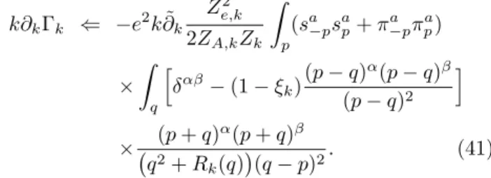
FIG. 1. The diagram that is responsible for the flow of the scalar wave function renormalization factor Zk. Solid lines refer to the scalar (and pseudoscalar) fields, while the wig- gly one is the gauge propagator. No tensor structure is in- dicated explicitly. In the regularization proposed here, the gauge propagator is not regulated.

ing for in this gauge is remarkably simple: apart from a small catch one need not regulate the gauge field, Ai, only the scalars, i.e.,s^a andπ^a. We will not discuss it in detail, but it turns out that the other choice, correspond- ing to R2, is also simple; there one associates regulators, as usual, to all dynamical variables,Ai,s^a, andπ^a.

There are at least two ways to perform the calculation of k∂_kZ_k, leading to identical results. One way is to brute force calculate the corresponding terms in (5), but it is simpler to use diagrammatics. Since Tr log of the propagator is the sum of one-loop diagrams, one needs to evaluate only one graph, shown in Fig. 1. Not regulating the gauge field, we get the following contribution into k∂kΓk:

k∂_kΓ_k ⇐ −e²k∂˜_k Z_e,k² 2ZA,kZk

Z

p

(s^a_−ps^a_p+π^a_−pπ_p^a)

× Z

q

h

δ^αβ−(1−ξk)(p−q)^α(p−q)^β (p−q)²

i

× (p+q)^α(p+q)^β q²+R_k(q)

(q−p)². (41)

Neglecting anomalous dimensions and considering only the O(p²) terms in the q integral (the mass flow, i.e., terms with∼p⁰, is not interesting), we arrive at

p²k∂_kZ_k =e² 4Z_e,k² ZA,kZk

Z

q

k∂_kR_k(q) (q²+Rk(q))²

×1−ξk−x²+ 3ξkx²

q² p², (42) where x= ˆp·q. As announced in Sec. II, we work withˆ the optimal regulator,R_k(q) = (k²−q²)Θ(k²−q²), and get

k∂kZk =k^D−4Ω_D D

8e²_kZ_k

(D −2)(D −1 +ξk(3− D)),(43) where we have also introduced the flowing charge; see above (3),e_k=eZ_e,k/Z_kZ_A,k^1/2.

Note that (43) does not agree with the corresponding result of [11], but this is only because we are working in a different gauge. We will see that once combined with the flowk∂_k(g_1,kZ_k²) [see (34)], the coupling flowk∂_kg_1,k is consistent with that of [11] (note that there no second

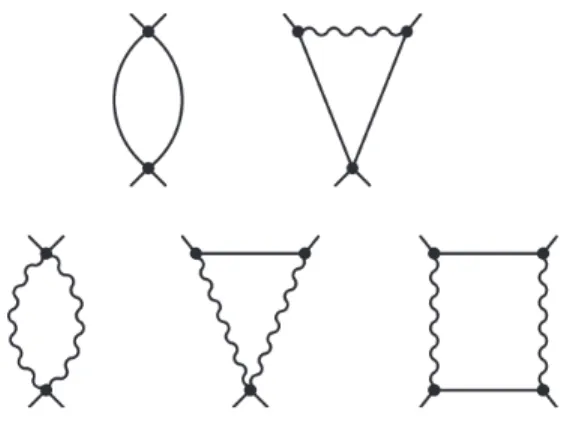
FIG. 2. Diagrams that contribute to the flow of the gauge wave function renormalization factor,ZA,k. Solid lines mean scalar (and pseudoscalar) propagators, while the wiggly ones refer to the gauge field.

coupling,g_2,k, was present).

B. Gauge wave function renormalization The calculation of the gauge wave function renormal- ization is completely identical to that of [11]. Two dia- grams need to be taken into account; see Fig. 2. We just review the result here: the flow ofZ_A,k is

k∂kZA,k=−k^D−4ΩD

D

16de²_k

D+ 2ZA,k, (44) and it turns out that even though one expects from the ansatz (2) the combination

k∂k

h ZA,k

Z Ai

2 (−∂²δij+ (1−ξ_k⁻¹)∂i∂j)Aj

i (45) to emerge in the rhs of (3), one actually gets from the two diagrams above

k∂k

h ZA,k

Z Ai

2 (−∂²δij+D −2

2 ∂i∂j)Aj

i

. (46) If D 6= 4, this selects only one gauge parameter that is consistent,

ξ_k≡2/(4− D). (47) For D = 4, any choice is allowed, as long as the gauge fixing parameter follows the flow of the gauge wave func- tion renormalization, i.e.,ξk ∼ZA,k, in accordance with perturbation theory. We will see that in this particular dimension the β-functions do not depend on the actual value ofξ_k after all. We also note that the induced mass of the gauge field, which comes from the momentum inde- pendent part of the two diagrams of Fig. 2, is completely dropped. It has been shown that neglecting it is not of any concern, since once adjusted at the UV scale, this term completely dies out in the IR and has no relevance [10, 11].

Also note that, as announced in the beginning of Sec.

III, the scalar mass was set to zero, µk ≡ 0. Had we not imposed this requirement, the result (46) would not be compatible with (45) for any gauge fixing parameter.

It would be interesting to further analyze the source of this violation of gauge symmetry, but here we leave it for future studies.

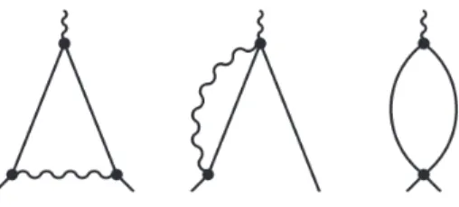
FIG. 3. Diagrams (with zero external momenta) that con- tribute to the flows of the coupling constants g1,k and g2.k. Solid lines refer to the scalar (and pseudoscalar) fields, while the wiggly one is the gauge propagator. No tensor structure is indicated explicitly.

C. Charge corrections to the coupling flows We make use of diagrammatics once again; see Fig. 3.

The first diagram is already done, as the whole previous section was devoted to analyze that very piece; the re- sults are summarized in (34) and (35). (Note that we do not differentiate the tensor structure in the diagrams, we only draw them for topological distinction.) The sec- ond piece is responsible for the O(g_1,ke²_k) and O(g_2,ke²_k) terms in the coupling flows. These type of terms lead to the following contribution into k∂kΓk:

k∂_kΓ_k ⇐k∂˜_k e²Z_e,k² 6Z_kZ_A,k

Z

x

(s^as^b(V_k,ss⁰⁰ )_ab+π^aπ^b(V_k,ππ⁰⁰ )_ab +π^as^b(V_k,πs⁰⁰ )ab+s^aπ^b(V_k,sπ⁰⁰ )ab)

× Z

q

1 (q²+Rk(q))²

1 q²

δ^αβ−(1−ξk)q^αq^β q²

q^αq^β,

(48) where the V_k⁰⁰ matrix can be built up from the A and B matrices, see definitions in (13) and (14), and useful formulas in Appendix B. Neglecting the anomalous di- mension in the rhs of (48), we get

Z

x

−ΩD

D k^D−48ξke²_kZ_k²

×

g_1,k|Tr (Φ^†Φ)|²+g_2,kTr (Φ^†ΦΦ^†Φ) . (49) This result shows that only those four point operators appeared that are allowed by the Lagrangian, therefore, the RG flow is closed.

Finally, we analyze theO(e⁴_k) contribution to the cou- pling flows. The last three diagrams of Fig. 3 need to be evaluated. One immediately notes that if we wish to stick to the regularization, where the gauge propagators are not regulated, then we run into a divergence coming from the first diagram of the second line in Fig. 3. We

have no choice but to restore the gauge regulator, and then the diagrams lead to the following contributions to k∂kΓk, respectively:

• k∂˜k

−_4Z^Z4e,k2 ^e4 kZ_A,k²

R

x(s^as^a+π^aπ^a)²R

q 1 (q²+R_k(q))²

×h

δ^αβ−(1−ξ_k)^qα_q2^qβih

δ^βα−(1−ξ_k)^qβ_q^q₂^αi ,

• k∂˜k Z⁴_e,ke⁴ 2Z²_kZ_A,k²

R

x(s^as^a+π^aπ^a)²R

q 1 (q²+Rk(q))³

×h

δ^αβ−(1−ξk)^qα_q2^qβ

ih

δ^βγ−(1−ξk)^qβ_q^q2^γ

i q^γq^α,

• k∂˜k

−_4Z^Z4e,k2 ^e4 kZ_A,k²

R

x(s^as^a+π^aπ^a)²R

q 1 (q²+R_k(q))⁴

×nh

δ^αβ−(1−ξk)^qα_q2^qβ

i q^αq^βo²

.

The sum of these three diagrams turn out to be Z

x

4

D(D −1) +ξ_k²h4

D − 12

D+ 2+ 8 D+ 4

i

×Ω_Dk^D−4Z_k²e⁴_k|Tr (Φ^†Φ)|². (50) The coefficient of theξ²_k term does not cancel, except for D= 4. Had it canceled, it would have led to a compati- ble result with [11] in theRξ gauge. The problem here is that the momentum dependent scalar (or pseudoscalar)- gauge vertices should also be regulated, because consis- tency would require to have regulated momenta flowing through all vertices, once the propagators entering them contain the regulator. A suitable vertex regularization can be achieved by adding the following off diagonal com- ponents to the regulator matrix:

R_k,Aαπ(q) =−iZ_e,ke(kqˆ^α−q^α)Θ(k²−q²)˜σ^a,(51a) Rk,Aασ(q) =iZ_e,ke(kˆq^α−q^α)Θ(k²−q²)˜π^a. (51b) This is a perfectly legitimate regulator contribution, quadratic in the dynamical variables, as ˜σ^a and ˜π^a are meant to be nondynamical, homogeneous fields, which are supposed to be set equal to the actual (homogeneous) value of σ^a and π^a, where the effective action is evalu- ated. In accordance with (51), by introducing the nota- tionq^α_R = ˆq^α[q+ (k−q)Θ(k²−q²)], the diagrams take the form of (the first one does not change)

• k∂˜k

− ^Z

4 e,ke⁴ 4Z²_kZ_A,k²

R

x(s^as^a+π^aπ^a)²R

q 1 (q²+R_k(q))²

×h

δ^αβ−(1−ξ_k)^qα_q2^qβih

δ^βα−(1−ξ_k)^qβ_q^q₂^αi ,

• k∂˜_k ^Z

4 e,ke⁴ 2Z²_kZ_A,k²

R

x(s^as^a+π^aπ^a)²R

q 1 (q²+Rk(q))³

×h

δ^αβ−(1−ξk)^qα_q2^qβ

ih

δ^βγ−(1−ξk)^qβ_q^q2^γ

i q_R^γq_R^α,

• k∂˜k

−_4Z^Z4e,k2 ^e4 kZ_A,k²

R

x(s^as^a+π^aπ^a)²R

q 1 (q²+R_k(q))⁴

×nh

δ^αβ−(1−ξ_k)^qα_q2^qβi q^α_Rq_R^βo²

.

Using the equality of the unit vectors, ˆq^α_R = ˆq^α, and performing all differentiations and integrations, the ξk

dependence indeed cancels, and the sum of the three di- agrams contributing to the flow of the effective action becomes

k∂_kΓ_k⇐ Z

x

Ω_D

D k^D−44(D −1)Z_k²e⁴_k

|Tr (Φ^†Φ)|². (52) Collecting all contributions from (38), (39), (49), and (52), we get

k∂k(Z_k²g1,k) =Z_k²Ω_D D k^D−4h

8(d+ 4)g²_1,k+ 16NTdg1,kg2,k

+12C2(A)NTg_2,k² −8ξke²_kg1,k+ 4(D −1)e⁴_ki , (53) k∂_k(Z_k²g_2,k) =Z_k²Ω_D

D k^D−4h

48g_1,kg_2,k

+ (20NTd−24C2(A))g²_2,k−8ξke²_kg2,k

i .(54) If we set g_2,k ≡ 0, using the flow of Z_k, we get back our earlier results for the β functions (see below) for N complex scalar fields with U(1) gauge symmetry (d = N) [11], obtained in theRξ gauge. As also discussed in Sec. IVD, in that earlier approach, we used a regulator, which was formulated in terms of eigenmodes and not the original field variables. Now what we see is that in the usual covariant gauge, identical results can only be achieved if the regulator is constructed more like at the level of diagrams. Gauge propagators have to contain a regulator where it was inevitably necessary (to avoid IR divergences), but not if the diagrams at the given order do make sense without it.

That is to say, it is allowed to switch between regular- ization schemes at different levels of the calculations, as long as the associated regulator functions are legitimate and do not lead to divergences. This could be surprising at first sight, as in the FRG approach, one usually de- fines the regulator before evaluating any projection of the flow equation. But since any legitimate regulator repre- sents a construction of the scale evolution of the effective action, one may regard switching between regularization schemes as a part of the employed approximation. Since we get the very same results this way compared to the one that associates regulators (in advance) to eigenmodes, we believe that our current approach is justified.

D. β functions and fixed points

Now we analyze theβfunctions ofg_1,k,g_2,k, ande²_kand search for fixed points. The β functions are defined as the flow of dimensionless couplings, i.e., ¯g1,k=g1,kk^D−4,

¯

g_2,k=g_2,kk^D−4, ¯e²_k=e²_kk^D−4. By definition, they are β_g1 ≡k∂_k¯g_1,k

= (D −4)¯g_1,k+k^D−4

Z_k² k∂_k(Z_k²g_1,k)−2¯g_1,kk∂_kZ_k Zk

,

(55) βg₂ ≡k∂k¯g2,k

= (D −4)¯g2,k+k^D−4

Z_k² k∂k(Z_k²g2,k)−2¯g2,k

k∂kZk

Z_k . (56) As for the flowing charge, e¯²_k = k^D−4e²_k, e²_k = e²Z_e,k² /Z_k²Z_A,k, we have

β_e2 ≡k∂ke¯²_k

= (D −4)¯e²_k−¯e²_kk∂kZA,k

ZA,k

+ ¯e²_k Z_k² Z_e,k² k∂k

Z_e,k² Z_k²

.

(57) We assume that the Ward identity Ze,k = Zk is satis- fied, and thus the last term is zero. We will come back to this issue in Sec. IVE, but note that this is a particularly important point, as this last, anomalous term would com- pletely change the nature ofβe² had it not been dropped, and due to the fact thatD= 3, prevented the existence of fixed points with a finite charge for a small number of scalars. Using (43), (44), (53), (54), we get

βg₁ = (D −4)¯g1,k+ΩD

D n

8(d+ 4)¯g_1,k² + 16NTd¯g1,k¯g2,k

+ 12C₂(A)N_T¯g_2,k² + 8¯e²_k¯g_1,k(D −4)ξk−2(D −1) D −2

+ 4(D −1)¯e⁴_ko

, (58)

βg₂ = (D −4)¯g2,k+Ω_D D

n

(20dNT −24C2(A))¯g²_2,k + 48¯g_1,kg¯_2,k+ 8¯e²_kg¯_2,k(D −4)ξ_k−2(D −1)

D −2

o, (59) β_e2 = (D −4)¯e²_k+Ω_D

D 8d

D+ 2e¯⁴_k. (60) We see that inD= 4, theξdependence vanishes, but for D 6= 4, one needs to substitute (D −4)ξk → −2; see the calculation prior to Eq. (47).

There are various fixed points displayed as solutions of the coupled equations of (58), (59), (60). Analytic solutions are available, but we do not list them as they are too long. For chargeless (¯e_k ≡0) fixed points, there are always two solutions with ¯g1,k 6= 0, ¯g2,k = 0 (i.e., Gaussian and Wilson-Fisher), and if

36(C2(A))²+ 12C2(A)(4−3d)NT+d²N_T²>0,(61) then two new ones appear with ¯g1,k 6= 0, ¯g2,k 6= 0. For charged fixed points (¯e_k6= 0), inD= 3, there are always two fixed points, where ¯g_1,k 6= 0, ¯g_2,k = 0 (these are equivalent to the superconducting and tricritical fixed