Impacts of autonomous vehicles on the urban fundamental diagram
Qiong Lu1, Tamás Tettamanti1, István Varga1
1 Department of Control for Transportation and Vehicle Systems, Faculty of Transportation Engineering and Vehicle Engineering, Budapest University of Technology and Economics, Hungary
Abstract
In recent years, selfdriving cars are being introduced to streets, which generated significant attention and discussion. The widespread adoption of autonomous vehicles (AV) brings changes in several fields. One of the most exciting changes is presented by the effect that driverless cars bring to the wellknown traditional traffic model, the Macroscopic Fundamental Diagram (MFD). This is a key issue as MFD is a basic model for strategic traffic planning and also for realtime traffic control. In this paper therefore the impacts of autonomous vehicles that are relevant to the urban MFD are investigated through traffic simulation. The paper seeks the answer to a basic question, i.e. how the different percentage of autonomous vehicles among traditional vehicles and the autonomous driving levels influence the urban MFD. A detailed simulation study was carried with SUMO (microscopic traffic simulation software) in an artificial grid network.
Keywords: autonomous vehicles, percentage, autonomous driving levels, fundamental diagram, urban traffic, SUMO
1 Introduction
In our days and in the near future connected and automated vehicles transform our traditional transportation systems (SAE International, 2014; Szigeti et al., 2017). Therefore, the impact of autonomous transport must be properly investigated as it directly influences the traffic dynamics, the applicable control, as well as the methodologies for traffic network analysis and planning [1, 2].
An autonomous vehicle (AV) by definition is a vehicle that is capable of sensing its environment and navigating without human input. Based on the amount of driver intervention and attentiveness required, the autonomous driving is classified into six different levels by the Society of Automotive Engineers (SAE) international. The SAE international delivered a harmonised classification system for Automated Driving Systems (ADS), specifically SAE J3016 Taxonomy and Definitions for Terms Related to OnRoad Motor Vehicle Automated Driving Systems (see Table 1) [3].
Experience with the availability and deployment of previous vehicle technologies can be used to forecast the AVs implementation. The penetration of driverless cars depends on both availability and user acceptance of the technology. Based on some widely accepted basic principles [4], six scenarios with different penetration in each autonomous driving level are studied in this paper.
Table 1. The levels of automation defined in SAE J3016 [3]
Level 0 – No automation
The fulltime performance by the human driver of all aspects of the dynamic driving task, even when enhanced by warning or intervention systems
Level 1 – Driver Assistance
The driving modespecific execution by a driver assistance system of either steering or acceleration/deceleration using information about the driving environment and with the expectation that the human driver performs all
remaining aspects of the dynamic driving task.
Level 2 – Partial Automation
The driving modespecific execution by one or more driver assistance systems of both steering and acceleration/deceleration using information about the driving environment and with the expectation that the human driver performs
all remaining aspects of the dynamic driving task.
Level 3 – Conditional Automation
The driving modespecific performance by an automated driving system of all aspects of the dynamic driving task with the expectation that the human drivers
respond appropriately to a request to intervene.
Level 4 – High Automation
The driving modespecific performance by an automated driving system of all aspects of the dynamic driving task, even if a human driver does not respond
appropriately to a request to intervene.
Level 5 – Full Automation
The fulltime performance by an automated driving system of all aspects of the dynamic driving task under all roadway and environmental conditions that can
be managed by a human driver.
The Macroscopic Fundamental Diagram (MFD) of traffic flow is practically a set of diagrams that gives relationships among the traffic flow ( ), the traffic density ( ) and the space mean speed ( ) [5]. The MFD can be used to define the capacity and thus the service level of a road system.
Moreover, the MFD describes traffic dynamics when applying inflow regulation or speed limits. Fundamental diagram consists of three different (two dimensional) graphs: flowdensity, speedflow, and speeddensity. All the graphs are related by the fundamental equation:
(1)
The fundamental diagram can be derived by plotting of field data points and using appropriate curve fitting to the scatter plots. MFD can also be applied for urban or metropolitan areas as proposed by [6]. The concept of urban MFD has been widely investigated during the past decades, e.g. [710].
The aim of this work is to study the potential impact of autonomous vehicles on the classical urban MFD.
2 Method
In this research, there are two main parameters to investigate in relationship with the fundamental diagram, i.e. the impact of penetration (percentage of AVs in the whole traffic flow) and autonomous driving level.
The work has been carried out with SUMO microscopic traffic simulation software by using different car types and percentages. The simulations were run in a grid network considering each group of these new parameters. The traffic volume of the links as well as the throughput of the whole network were measured in the simulator virtually. All measures of the MFD can be obtained from SUMO’s edgeData which represents macroscopic linklevel measurement practically. The results were evaluated in order to understand the evolution of the different scenarios and reveal the relationships between network capacity, percentage of autonomous car as well as autonomous driving level.
Regarding the MFD, networklevel and linklevel fundamental diagram can be distinguished, both by using Eq. (1). The first one models the throughput of the traffic network per hour:
(2)
where is the number of vehicles that pass the network. is the average density of the network, and it simply equals to the known total number of vehicles in the network divided by the total link kilometres of the road network, i.e.
(3)
where is the length of link , is the number of links [5,10].
The second approach interprets the MFD of one single road link of the network, i.e.
(4)
where is the flow, means the density, defines the mean velocity, and is the flow on link .
In our work, fundamental diagrams were modelled as polynomials. Thus, the points of the simulation results were approximated with cubic polynomial curve fitting (the fitting curve was constrained to cross the original):
(5)
where, , , are polynomial coefficients.
3 Simulation Study and Evaluation
In order to analyse the effect of automated and autonomous technology a detailed simulation study was carried with SUMO microscopic traffic simulator.
3.1 Network setup and scenarios
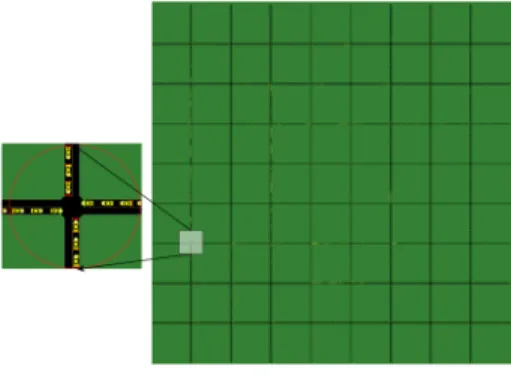
As shown in Fig. 1, a grid traffic network was constructed, designed to represent common situation on the urban road network. The applied network was an 8×8 grid, i.e. 64 intersections in the network. The length between adjacent node was 500 meters. The network edges were bidirectional road links with single lanes. A traditional “time gap based” traffic signal method was applied (builtin tool of SUMO [11]). This control scheme switches to the next phase after detecting a sufficient time gap between successive vehicles in order to achieve a better distribution of greentime among phases dynamically [12].
Figure 1. Grid test traffic network
As the aim of this work is to investigate potential impacts of driverless cars on road network performance, a straightforward approach to autonomous vehicles fleet penetration has been taken. This is based upon some basic principles that are widely accepted:
• at low market penetration, technical capability is limited (for example, to driver assistance which mean low autonomous driving level);
• as market penetration increases, consumer confidence also augments and better use of connected and automated technology prevail [4].
Fig. 2 shows an example projection for the increasing technical capability of AVs overtime. Technological change is usually marked by early adopters prior to full saturation. The scenarios for AV deployment should reflect this.
Figure 2. Future states of availability and user acceptance [4]
Measurements in one link and in the whole network were realized. The modelled scenarios are summarised in Table 2.
Table 2. The scenarios used in this simulation Scenario
nr.
Scenarios Ratio of traditional
cars
AV penetration composition Level 1 Level 2 Level 3 Level 4 Level 5
1 Base 100% 0% 0% 0% 0% 0%
2 25% penetration 75% 15% 5% 5% 0% 0%
3 50% penetration 50% 25% 10% 10% 5% 0%
4 75% penetration 25% 25% 20% 15% 10% 5%
5 100% penetration 0% 15% 20% 20% 25% 20%
6 Upper bound 0% 0% 0% 0% 0% 100%
3.2 Autonomous vehicle modelling methodology
Default SUMO parameters have been modified in order to model a plausible future for AVs. In this paper, the default car following model was applied (Krauss Model). The parameter selection is related to longitudinal movement, acceleration, deceleration and gap acceptance. These behaviours are formalised as parameters in the carfollowing model of SUMO. The implemented model follows the idea as that let vehicles drive as fast as possibly while maintaining perfect safety (always being able to avoid a collision if the leader starts braking within leader and follower maximum acceleration bounds). The following list shows the editable parameters of the Krauss Model:
• Mingap: the offset to the leading vehicle when standing in a jam (in m).
• Accel: The acceleration ability of vehicles of this type (in m/s2).
• Decel: The deceleration ability of vehicles of this type (in m/s2).
• Emergency Decel: The maximum deceleration ability of vehicles of this type in case of emergency (in m/s2).
• Sigma: The driver imperfection (between 0 and 1).
• Tau: The driver’s desired (minimum) time headway (reaction time) (in s).
For level 0 the default values were taken for all parameters. But the emergency deceleration was set to 8 m/s2. This value is based on the study of [13]. For other autonomous driving levels, the deceleration and the emergency deceleration remained the same, considering the safety.
For the level 2 and level 5, the mingap, acceleration, time headways were taken from [4]. For level 1, the values of these items were set as the average value of level 0 and level 2. For the level 3 and level 4, the values of these items were changed linearly between level 2 and level 5. The driver imperfection for level 5 and level 4 was set to 0, because these levels do not need human driver’s
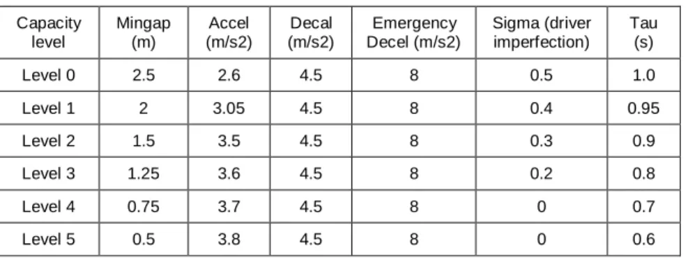
intervention. It was assumed to be 0.4, 0.3 and 0.2 for level 1, level 2 and level 3, respectively. The parameters for all levels are tabulated to Table 3.
Table 3. Variables in SUMO carfollowing model Capacity
level
Mingap (m)
Accel (m/s2)
Decal (m/s2)
Emergency Decel (m/s2)
Sigma (driver imperfection)
Tau (s)
Level 0 2.5 2.6 4.5 8 0.5 1.0
Level 1 2 3.05 4.5 8 0.4 0.95
Level 2 1.5 3.5 4.5 8 0.3 0.9
Level 3 1.25 3.6 4.5 8 0.2 0.8
Level 4 0.75 3.7 4.5 8 0 0.7
Level 5 0.5 3.8 4.5 8 0 0.6
3.3 Simulation results
The main simulation results are provided by Figs 34. and Table 4. From the results for the whole network, one can see that from scenario 1 to scenario 6 the capacity of the whole network is increasing and the critical density varies.
Scenario 6 has the largest critical density straightforwardly. The same tendency can be found in whole network for critical density and capacity that going up in the beginning, then decreasing, roaring up at the end.
From the results for one single link, one can see that the capacities for scenario 1, 2, 3 and 4 are similar and relatively smaller, and the capacities for scenario 5 and 6 are bigger and have an increasing trend. The same change can be found on the critical densities.
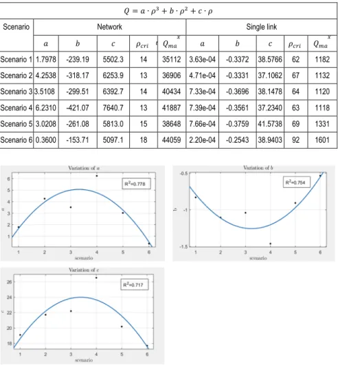
Fig. 4. shows the coefficients of the fitting curves which are fitted with quadratic polynomials. From the changes of the coefficients, one can see, the goodness of fitting is relatively high which means the total variation of the coefficients can be explained by the quadratic polynomials well.
Figure 3. Simulation results for the whole network and a single link
Table 4. Network overall fitting result
Scenario Network Single link
!" #
$
%
!" #
$
%
Scenario 1 1.7978 -239.19 5502.3 14 35112 3.63e-04 -0.3372 38.5766 62 1182 Scenario 2 4.2538 -318.17 6253.9 13 36906 4.71e-04 -0.3331 37.1062 67 1132 Scenario 3 3.5108 -299.51 6392.7 14 40434 7.33e-04 -0.3696 38.1478 64 1120 Scenario 4 6.2310 -421.07 7640.7 13 41887 7.39e-04 -0.3561 37.2340 63 1118 Scenario 5 3.0208 -261.08 5813.0 15 38648 7.66e-04 -0.3759 41.5738 69 1331 Scenario 6 0.3600 -153.71 5097.1 18 44059 2.20e-04 -0.2543 38.9403 92 1601
Figure 4. The variations of the fitted polynomial coefficients (network level) together with the regression curves
4 Conclusion
The effect of automated and autonomous vehicles to the urban MFD have been analysed through microscopic traffic simulation. A thorough simulation study was fulfilled in a grid traffic network. The results justified some regularity in the change of the urban MFD (network and link level as well) along with the autonomous technology evolution. The results are also important from the point of view of practical traffic engineering as the fundamental diagram is a common modelling
approach when planning or analysing a road network. Therefore, one should take these changes into consideration in the future.
5 Acknowledgement
The research work was supported by the Hungarian Government and cofinanced by the European Social Fund (EFOP3.6.3VEKOP16201700001: Talent Management in Autonomous Vehicle Control Technologies) and by the János Bolyai Research Scholarship of the Hungarian Academy of Sciences.
References
[1] L. Kisgyörgy, G. Vasvári: Analysis and observation of road network topology, 19th International Conference of Hong Kong Society for Transportation Studies, Hong Kong, December 2014,
[2] Sz. Szigeti, Cs. Csiszár, D. Földes: Information Management of DemandResponsive Mobility Service Based on Autonomous Vehicles, Procedia ENGINEERING 187: pp.
483491. 2017.
[3] S. O.R. A. V. S. Committee et al., “Taxonomy and definitions for terms related to on
road motor vehicle automated driving systems,” SAE Standard J3016, pp. 01–16, 2014.
[4] A. Ltd, “Research on the impacts of connected and autonomous vehicles (cavs) on traffic flow research on the impacts of connected and autonomous vehicles (cavs) on traffic flow,” tech. rep., Department for Transport, 2016.
[5] J. C. Williams, H. S. Mahmassani, S. Iani, and R. Herman, “Urban traffic network flow models,” Transportation Research Record, vol. 1112, pp. 78–88, 1987.
[6] J. Godfrey, “The mechanism of a road network,” Traffic Engineering & Control, vol. 8, no. 8, 1969.
[7] H. Mahmassani, J. C. Williams, and R. Herman, “Performance of urban traffic networks,” in Proceedings of the 10th International Symposium on Transportation and Traffic Theory, pp. 1–20, Elsevier Amsterdam, The Netherlands, 1987.
[8] C. F. Daganzo, “Urban gridlock: Macroscopic modeling and mitigation approaches,”
Transportation Research Part B: Methodological, vol. 41, no. 1, pp. 49–62, 2007.
[9] M. KeyvanEkbatani, M. Papageorgiou, and I. Papamichail, “Perimeter traffic control via remote feedback gating,” ProcediaSocial and Behavioral Sciences, vol. 111, pp. 645–653, 2014.
[10] A. Csikós, T. Tettamanti, and I. Varga, “Macroscopic modeling and control of emission in urban road traffic networks,” Transport, vol. 30, no. 2, pp. 152–161, 2015.
[11] “Simulation/traffic lights,” http://sumo.dlr.de/wiki/Simulation/Traffic_Lights, 14 March 2018.
[12] D. Krajzewicz, J. Erdmann, M. Behrisch, and L. Bieker, “Recent development and applications of SUMO Simulation of Urban MObility,” International Journal On Advances in Systems and Measurements, vol. 5, pp. 128–138, December 2012.
[13] N. Kudarauskas, “Analysis of emergency braking of a vehicle,” Transport, vol. 22, no. 3, pp. 154–159, 2007.