2D vs. 3D Numerical Approaches for Fish Habitat Evaluation of a Large River — Is 2D Modeling Sufficient?

(1)

Cite this article as: Füstös, V., Erős, T., Józsa, J. "2D vs. 3D Numerical Approaches for Fish Habitat Evaluation of a Large River — Is 2D Modeling Sufficient?", Periodica Polytechnica Civil Engineering, 65(4), pp. 1114–1125, 2021. https://doi.org/10.3311/PPci.17788

2D vs. 3D Numerical Approaches for Fish Habitat Evaluation of a Large River — Is 2D Modeling Sufficient?

Vivien Füstös^1*, Tibor Erős², János Józsa^1,3

1 Department of Hydraulic and Water Resources Engineering, Faculty of Civil Engineering, Budapest University of Technology and Economics, H-1521 Budapest, P.O.B. 91, Hungary

2 Balaton Limnological Research Institute, H-8237 Tihany, Klebelsberg Kuno u. 3., Hungary

3 MTA-BME Water Management Research Group

* Corresponding author, e-mail: fustos.vivien@emk.bme.hu

Received: 04 January 2021, Accepted: 18 June 2021, Published online: 19 July 2021

Abstract

Computational Fluid Dynamics is an effective tool for assessing non-present conditions, thus also in habitat evaluation within ecohydraulics. Deciding whether to apply a one-, two- or three-dimensional numerical approach, is an optimization that needs to be performed by every task, given the capability and the demands of specific approaches. In this paper we compare the utility of two- dimensional (2D) versus three-dimensional (3D) hydrodynamical simulations for ecohydraulic purposes. The basis of the comparation were 1) three simulated abiotic variables: water depth, depth averaged flow velocity and bed material composition, and 2) an overall performance in a meso-scale fish habitat evaluation, based on the simulated three variables. The biotic parameters for the models were the habitat suitability curves of three fish species, the Danube streber (Zingel streber), the round goby (Neogobius melanostomus) and the white bream (Blicca bjoerkna). We found that in terms of ecohydraulic utilization, the 2D approach performed sufficiently to simulate the hydrodynamics of a large river. The errors originating from the 3D-2D simplification yielded negligible differences in habitat evaluation, and the agreement in the habitat suitability indices calculated from the simulated metrics was satisfactory.

Henceforth, the theory was turned into an application as we performed habitat mapping on a 100 km long, Hungarian reach of the Danube River, with the abiotic parameters resulting from a 2D hydrodynamical simulation. The possibility of simplifying the approach from 3D to 2D provides a cost-efficient numerical tool at larger scales for ecohydraulic studies, and especially for evaluating habitat suitability of riverine fish.

Keywords

ecohydraulics, computational fluid dynamics, habitat suitability indices, SSIIM, AdH, Danube streber, round goby, white bream

1 Introduction

Through the need for irrigation, hydraulic engineering has accompanied humanity since antiquity [1]. Taking into account of the continuity and safety of aquatic environments started first on a local scale in the 19^th century (e.g., a patent on a fish ladder in Canada is dated to 1880 [2]). The global awareness has been increasing in the last 20–30 years, establishing new research fields, such as ecohydraulics.

The aim of this field is to describe relations between biotic and abiotic parameters of the aquatic environment.

Fish habitat evaluation is a typical task in ecohydraulics, suitable for impact analysis of hydraulic engineering inter- ventions [3–5]. It may be performed at various scales, by various methods, and targeting several habitat types, i.e.:

feeding, nursing, sheltering etc., as well as general habitats.

A few methods of habitat evaluation, related to this paper,

follow. Microhabitat description (e.g., in [6, 7]) is based on fish abundance and locally measured specific hydro-morphological variables. The preferences of a species are determined for discrete intervals of the hydro-morphological parameters, resulting in habitat suitability indices (SI).

These indices can be interpreted as continuous habitat suitability functions, if the discrete intervals are aggregated to a larger range of values. The habitat suitability functions may be applied for evaluating regions of the aquatic environment, creating habitat suitability maps [8]. By mesohabitat evaluation (e.g., in [7, 9]) characteristic habitat types (e.g., pool, riffle, run, etc.) are defined based on specific parameters, and fish sampling is performed afterward, specifically on the appointed areas. Thus, preferences are interpreted on these specific habitat types.

(2)

The micro and meso prefixes refer to the scale of the approach (pointwise and areal, respectively). Bringing the scales closer to each other or upscaling is a challenge [10], although a combination of the two processes complete each other and may be efficient on large rivers for example [11].

Data collecting is essential prior to fish habitat evaluation and divides into two parts: abiotic data includes hydro-morphological and water quality metrics etc., and biotic data covers density, distribution of specific fish species. Fish abundance data may be collected by remote sensing [12] or by using classic fishing methods (e.g., trawl- ing, trapping, or electrofishing [13–15]). Abiotic metrics may be acquired via field survey and — with increasing efficiency and certainty — also remote sensing. However, caution and preferably a combination of the two is recom- mended when investigating hydro-morphologically com- plex systems [16].

In cases, when a field survey of the aquatic environment is not possible (e.g., for non-present conditions), researchers rely on computational fluid dynamic methods. Considering the capacity of approaches with various dimensionality and the metrics generally deemed important for habitat evaluation (e.g., bed shear stress), 2D hydrodynamic simulations are commonly applied for ecohydraulical purposes (e.g., in [3, 5, 8, 9, 11]). Notwithstanding, there has been a precedent for the use of 1D computation, in which the results of one cross-section (e.g., mean velocity value) were subdivided manually between verticals, thus expanding results to two dimensions [17]. Comparing 2D and 3D, it was found that near-bed conditions can be estimated more reliably by the latter. However, less effort is needed for a 2D computation [18], besides calibrating certain correction-factors for the computation (e.g., setting a factor for the effect of secondary circulation, or correcting depth-averaged flow velocity with vertical velocity profile) may reduce the differences between the two approaches [18–21]. While the flow conditions can usually be sufficiently described with a depth-averaged (2D) approach, the relevance of vertically interpreted hydrodynamics increases in the case of ecohydraulic analyses [22, 23].

To sum up, simplification is dependent on the object of the task. The 3D approach is more reliable reproducing near-bed conditions, although its cost-efficiency decreases with the expansion of the model domain. Running a 2D simulation can be more efficient at large spatial or tempo- ral scales. Targeting such an extended reach as study site

yields the following question, which, to our knowledge, has not yet been addressed: Is a depth-averaged 2D approach sufficient for habitat evaluation of large river reaches?

The goal of this study is first to compare the results of 2D versus 3D simulations on 5–7 km long model domains.

This aims to reveal the extent of the error that results from the simplification. These geometries are two simplified test channels and an existent river reach (comparative study). Our second goal is to establish habitat suitability maps of three fish species for a ca. 100 km long study site (the Upper-Hungarian reach of the Danube River), by char- acterizing the general habitat use patterns of the species.

A novel habitat mapping method is adapted here, which combines the results of numerical simulations and habitat suitability functions [8]. Due to the extended length of the model domain, and based on our findings in the former section, we perform the simulations in 2D (applied study). The three fish species are the endemic and protected Danube streber (Zingel streber), the invasive round goby (Neogobius melanostomus) and the commercially important white bream (Blicca bjoerkna). We consider the three targeted categories above to be important in environmental management.

2 Study site

2.1 Comparative study

The model domains of the comparative study are two arbitrary designed schematic channels and a reach of the Danube River.

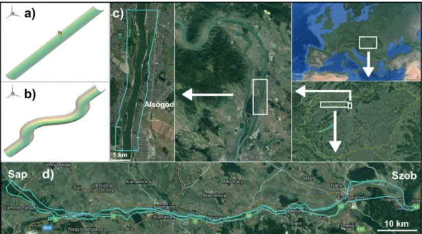
Channel A is a simplified 5,000 m long and 400 m wide, straight geometry with a parabolic profile crosswise (Fig. 1(a)). It has a 130 m long, 5 m wide, transversal groin, 2,000 m away from the uppermost cross section. The crest level of the groin is 3 m. The deepest level of the bed at the upstream boundary section is -2 m. The slope of the channel is 5 cm km^–1, thus the deepest level of the bed at the downstream boundary section is -2.25 m. (These are not above sea levels.)

Channel B is also a simplified 5,000 m long and 400 m wide meandering geometry, which has no groin (Fig. 1(b)).

In terms of levels and slope, it is identical to Channel A.

Channel A and B were both built with a mesh constructing software (see in Section 3.1). The reason of constructing these schematic, elementary geometries was to reproduce phenomena that are specific to groins and meandering reaches. Thus it was possible to examine the plain 2D and 3D representations of them.

(3)

Channel C is an existent river reach, the same site discussed in [7] and [8] (Fig. 1(c)). This is a free-flowing, ca. 7,000 m long section of the River Danube, located at Alsógöd, Hungary, between rkm 1,672 and 1,665. The width of the main channel is 400 m, the mean depth is 4 m and the mean slope is 5 cm km^–1.

2.2 Applied study

The selected site of the applied study is a part of the Danube reach, which serves as a border for Hungary (HU) and Slovakia (SK), located between rkm 1,811 and 1,708, from Sap (SK) to Sob (HU), as shown in Fig. 1(d). The investigated free-flowing section is edged with groins, longitudi- nal training walls and islands and has a few mid-channel gravel bars and bottlenecks. According to the third Joint Danube Survey performed in 2013 [24], bed-material in the main channel shows a continuous transition from peb- bles to coarse sand. The width of the reach varies between 1,000 and 400 m due to the diverse distribution of islands and branches. The mean slope is 7 cm km^–1.

The population of fish is derived from previous sam- plings carried out by Erős et al. [13] and Szalóky et al. [14], both in the littoral and benthic zone of the Danube. For collecting fish, electrofishing gears and an electrified benthic frame trawl were used in the littoral zone and offshore, respectively. These two types of data collecting techniques complete each other regarding the spatial distribution of the samples. The largest samples in the littoral

zone belonged to the common bleak (Alburnus alburnus) and the round goby with thousands of specimens, while the white-finned gudgeon (Romanogobio vladykovi), the white bream and the Kessler's goby (Ponticola kessleri) also held considerable numbers.

The common bleak nearly disappeared in the benthic catches, supporting the literary fact that the species is most likely to be found near the water surface [25]. The round goby, compared to the other species, was found in an out- standing quantity, while only a few hundred individuals were equally present from the succeeding Danube streber, white-finned gudgeon, schraetzer (Gymnocephalus schraetser) and common zingel (Zingel zingel).

3 Materials

3.1 CFD of the comparative study

The 2D and 3D simulations were performed with the software Adaptive Hydraulics Modeling System, version 3.2 [26] (AdH) (e.g., in [27]) and Simulation of Sediment Movements in Water Intakes With Multiblock Option, version 2 [28] (SSIIM) (e.g., in [29–32]), respectively. Table 1 shows the most significant differences between the two solvers.

As Table 1 shows, bed shear stresses are not computed within the applied 2D model. Hence, this was calculated following the simulation, for each computational node with Eq. (1), which is based on the slope method for bed shear stress, supplemented by Manning's formula [33].

Fig. 1 The investigated domains of the study; a) Channel A of the comparative study, a schematic, straight, 5000 m long riverbed with a groyne;

b) Channel B of the comparative study, a schematic, meandering, 5000 m long riverbed; c) Channel C of the comparative study, a ca. 7000 m long reach of the Danube River; d) Model domain of the applied study, a ca. 100 km long reach of the Danube River. Background map: Google Earth

(4)

τ τ^bx ρ

by g n h u

v u v



 

 = 

 

 +

−

* * ²* * *

1

3 2 2 . (1)

Variables in Eq. (1):

• τ_bx and τ_by are bed shear stresses in x and y direction, respectively,

• h is water depth,

• u and v are depth-averaged velocity in x and y direc- tion, respectively,

• ρ and g are water density and gravitational accelera- tion, respectively,

• n is Manning's roughness value.

Bed material composition was defined for each node, using a bed shear stress based mapping method. This method applies relationships set up between the local bed shear stress values (from Eq. (1) in the 2D modeling) and bed material fractions, collected in the study reach in a previous research. A detailed description of the procedure can be found in [8], generally, the higher the bed shear stresses are, the coarser the simulated bed material composition is.

Surface-water Modeling System, version 11.0.04 [34]

(SMS) was used for mesh construction. The comparation of the 2D and 3D simulation was carried out by examining the difference in the nodal values. Hence, grid nodes (into which values are interpolated by visualization), whether of a structured or an unstructured grid, must match. For this reason, every grid we prepared was constructed with quadrilateral shaped cells, and then either left like that for a structured 3D grid, or split into two triangles by each cell for an unstructured 2D grid. SSIIM allows adaptive defining of horizontal cell layers for 3D grids, meaning the number of layers depends on current depth and may vary in space and time. The maximum number of layers was set to 11. At the end of the process, the 2D grids of Channel A and Channel B consisted of ca. 80,000 computation cells, while the 3D grids were composed of ca. 360,000 cells.

The cell number of the 2D grid of Channel C was ca.

52,000, while the 3D grid consisted of ca. 150,000 cells.

Simulations of the comparative study were carried out at low, mean and high water levels in each of the three channels, in both 2D and 3D approaches, which made 18 simulations altogether. The applied boundary conditions for the 2D and 3D simulations are listed in Table 2. Due to the short length of every channel, only one inlet and one outlet needed to be defined in every case.

Water depth boundary conditions for Channel A and Channel B in Table 2 were determined considering the crest level of the groin and the flow discharges, considering typical low, mean and high flow discharges of the Danube River. Calibration and validation were performed in [8] for Channel C. (Channel A and B are non-existent, simplified channels, the first step of what intended to be a series of Danube scaled test channels. However, as we obtained good results already on those, the series was not continued, we rather went on to examine Channel C.) 3.2 CFD of the applied study

The 2D simulations were performed with the above-mentioned software AdH. Grid (and elevations) for the computation was acquired in parts from the Executive Riverbed Management Plan [35], ready to use after combining the parts. The complete grid consisted of ca. 199,000 cells.

Simulations were carried out at three flow regimes: low and mean water level and a 100-year flood (Table 3). Of the several tributaries, four were deemed significant and were built in the model: Branch Mosoni-Danube (rkm 1,794), River Vág (rkm 1,766), River Garam (rkm 1,716) and River Ipoly (rkm 1,708). The applied boundary conditions are listed in Table 3. The flood conditions were obtained from the Executive Riverbed Management Plan [35]. The flow values of the Mosoni-Danube branch were adopted from its water-level control structure research [36], and the majority of the rest of the values from the design flood level research [37]. The negative discharge value for the Mosoni-Danube during flood conditions indicates the backwater effect of the Danube towards the tributary.

Table 1 Contrast of the two software by the most important features regarding this study

AdH SSIIM

Approach 2D 3D

Equations Shallow-water

equations Reynolds-averaged Navier- Stokes

Grid Unstructured

(triangles) Structured

(quadrilateral) Bed-shear stress Not computed Computed from the kinetic

energy of near-bed cells

Table 2 Boundary conditions for 2D and 3D simulations of the comparative study (w.l. = water level)

Boundary conditions

Channel A and Channel B Low w.l. Mean w.l. High w.l.

Inlet: Q [m³ s^–1] 1,100 2,200 5,000

Outlet: H [m] 2 3 5

Boundary conditions

Channel C

Low w.l. Mean w.l. 100-year flood

Inlet: Q [m³ s^–1] 1,150 1,690 6,100

Outlet: Z [m a. s. l.] 98.16 98.68 105.40

(5)

Calibration and validation were performed within [35], land-use coverages and their Manning's roughness values were adopted from there, as listed in Table 4.

3.3 Habitat suitability calculations

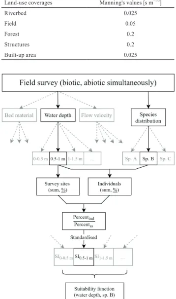
The abiotic metrics which were used for establishing SI functions were depth, depth-averaged flow velocity and bed material composition, which were simulated by hydrodynamic computations. The assessment of suitability criteria is based on 1) the occurrence of sample sites with hydrodynamic parameter values within different intervals and 2) the occurrence of the species on such sample sites.

The standardized proportion of these two percentile occur- rences yields the suitability index of a species for a specific interval of an abiotic parameter. The process is shown in Fig. 2, highlighted for water depth and a specific interval within. The procedure is the same for every discrete interval of water depth, and ultimately for every parameter (in grey). (For the sampling data used here, see also Erős et al. [13] and Szalóky et al. [14].) The values of the habitat suitability index range between 0 and 1, with the former indicating the habitat not to be suitable and the latter indicating the habitat to be optimal for a given species.

The aggregation of the indices for e.g., every 0.5 m interval of water depth yields the habitat suitability function for the whole range of sampled water depth.

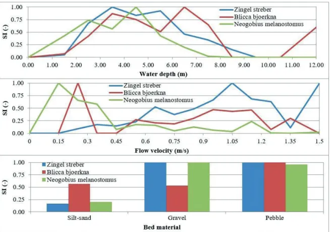
According to the former description, habitat suitability functions of the Danube streber, the round goby and the white bream for the three abiotic metrics were assessed, shown in Fig. 3. These functions are aggregations of habitat suitability indices quantified for intervals of hydrodynamic characteristics. For instance, in the case of the round goby, sites characterized by either mean water depth (2–5 m), or low velocities (<0.4 m s^–1), or with dominant pebble or gravel fractions are likely to be used as habitats.

There are three intervals with zero SI value on the water depth and flow velocity suitability functions (8.5–10.5 m;

0–0.15 m s^–1 and 0.35–0.45 m s^–1) of the white bream.

These are presumably caused by an insufficient sum of study sites characterized by the aforementioned intervals.

Therefore, these conditions cannot be labeled as com- pletely inadequate for the species.

4 Results and discussion 4.1 Comparative study

By the comparison of 2D and 3D approaches, values of the three simulated abiotic metrics used for establishing

Table 3 Boundary conditions for 2D simulations of the applied study (b. = boundary; w.l. = water level)

Boundary conditions Low w.l. Mean

w.l. 100-year flood

Discharge [m³ s^–1]

River Danube

(upper b.) 800 2,200 10,282

Branch Mosoni-

Danube 31 71 -336

River Vág 3 40 158

River Garam 7 30 135

River Ipoly 3 10 100

Water level

[m a. s. l.] River Danube

(lower b.) 99.63 101.31 107.67

Table 4 Land-use coverages and Manning's roughness values attached to them, used in the 2D model in the applied study

Land-use coverages Manning's values [s m^–1/3]

Riverbed 0.025

Field 0.05

Forest 0.2

Structures 0.2

Built-up area 0.025

Fig. 2 The procedure of assessing habitat suitability functions based on field sampling data, highlighted (in black) for one specific interval of one specific parameter. The method is the same for the parameters and

intervals in grey

(6)

habitat suitability functions were compared: water depth, depth-averaged flow velocity and bed shear stress (this latter was used for assessing bed material composition). The errors were elaborated by the subtraction of the simulated nodal values of the parameters. In case of the 3D model, the bottom layer nodal values were used. (Water depth and depth averaged flow velocity values are not dependent on the horizontal layer.) The bed shear stresses of the 2D model were calculated with Eq. (1). This process yielded absolute errors for the three variables, into every node, interpreted as error fields. A normalized mean error for each hydrodynamic variable for each flow regime was calculated as in Eq. (2).

∆ = 

 



=

−

=

− −

∑

i

∑

n

i i

n

dp n p ni 1

2 1

1 1

1

* * * (2)

Variables in Eq. (2):

• dp_i is the value at the i^th node in a specific error field,

• p_i is the value at the i^th node in the respective 2D variable field,

• n is the number of nodes.

Fig. 4 shows the calculated mean errors in the three channels (Channel A, B and C are labelled with their let- ters), for all flow regime scenarios (low, mean and high water level as 1, 2 and 3, respectively). Errors for Channel A and B remain under 13% in each scenario, although higher errors in Channel C indicate that the smaller differences result from the simplification. Among the three variables, the highest errors can be observed in the bed shear stress values. The greatest difference in general with 45–48%

belongs to bed shear stresses in Channel C. This is presumably due to the realistic morphology of the reach and also the different methods of computation (from kinetic energy of near-bed cells in 3D, and by Eq. (1) in 2D). Bed shear stress differences increase with the boundary discharge, which aligns with the findings of [38]. However, the differences we observed were ca. 10% less compared to that investigation.

These differences decreased when the results were applied for habitat evaluation. Habitat suitability functions of the Danube streber were paired with the respective results of both the 2D and 3D simulations for Channel C at the mean flow regime. The habitat suitability indices

Fig. 3 Habitat suitability indices of the three discussed fish species: the Danube streber (Zingel streber), the round goby (Neogobius melanostomus) and the white bream (Blicca bjoerkna) established for three abiotic metrics: water depth, depth-averaged flow velocity and bed material composition.

The closer to 1 the index is, the more preferred the habitat is, characterized by the parameter value. The underlying data is presented in [13] and [14].

(7)

for the three abiotic parameters were aggregated via averaging to form one general habitat suitability map by both approaches for the Danube streber, as Fig. 5 shows. To our knowledge, there is no data reported on the weights to be

used by averaging the suitability indices of the specific parameters, so the assumption of no weights was made.

These weights would represent the rank of the importance of the studied parameters for a specific fish species.

Fig. 4 Mean errors of abiotic parameters simulated by the 2D and 3D approaches on the three model domains in the comparative study. A, B, C - Channel A, B and C, respectively. 1 - low flow regime, 2 - mean flow regime, 3 - 100-year flood

Fig. 5 Habitat suitability maps of the Danube streber on Channel C at a mean flow regime, created by applying the habitat suitability indices on the simulated hydrodynamic parameters. Combined maps are the unweighted average of the three separate fields. An error field on the right is showing

the subtraction of 3D simulated SI values from 2D simulated SI values

(8)

The errors, which were high in the case of the bed shear stress attenuated in the process of assessing bed material composition. (This is due to the method, see in [8].) Henceforth, the averaging of habitat indices of specific parameters further reduced the difference yielding from the two approaches. This pattern also appears in the calculated errors of the separate and combined habitat maps.

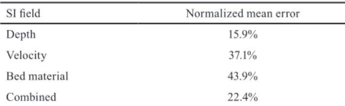
Table 5 shows a normalized mean error for each habitat suitability map (depth based velocity based, bed material based and combined), computed as in Eq. (2). The rela- tion of the habitat map errors regarding the three separate parameters is similar to what is displayed on the respective section of Fig. 4 (the values differ, due to the applied suitability functions). The aggregated habitat maps (in Fig. 5) originating from 2D or 3D numerical computation are considerably similar, the respective error is 22.4%.

The combined difference field on the right side of Fig. 5 shows that errors are greater near the shoreline. These are generally positive, which means that the 2D approach yielded higher suitability indices altogether. The pattern closely aligns with the differences of the separate bed material SI fields: the 2D approach simulated more suitable bed material composition in these areas. Bed material composition is derived from bed shear stresses, which tend to be higher in the case of the 2D simulation; and higher bed shear stresses yield coarser bed material composition. Thus, considering the respective part of Fig. 3, a coarser bed material composition means higher suitability indices for the Danube streber as an example presented on Fig. 5. Such differences in simulated bed material composition were located near the shoreline, while other areas were less affected.

Given the uncertainties in fish sampling and establishing habitat suitability criteria, we deemed the 22.4%

normalized mean error of the aggregated habitat maps acceptable. Therefore, as the 2D numerical approach is more cost-effective in many ways than the 3D approach;

a trade-off may be made of relying on 2D simulations

by considerably extended model domains. In contrary, if the near-bed conditions are at aim, and/or the study site is hydro-morphologically more diverse [8, 39], a 3D approach cannot be evaded.

The calculation method of bed shear stresses by the 2D approach generally yields higher values and thus indicates coarser bed material than the 3D computation. How this difference translates to habitat suitability is however unique to every species, as it depends on the suitability functions.

Thus, any similar studies require case- (or species-) sensi- tive interpretation of the results. An improved bed shear stress calculation method may reduce this uncertainty.

4.2 Applied study

Upon the former conclusion, habitat mapping of a 100 km long Danube reach was performed using the results of a 2D simulation. The used habitat suitability functions were assessed through statistical analysis of previous sam- plings. However, they may be represented as literature values [40] or so-called 'fuzzy rules' (e.g., IF water depth is high AND flow velocity is high, THEN habitat suitability is medium) [4, 41].

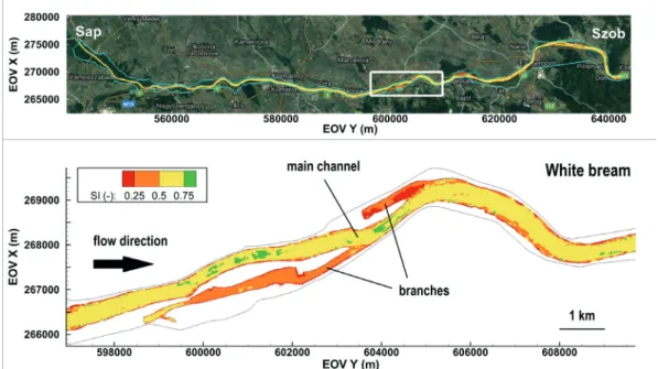
The upper panel of Fig. 6 shows a combined habitat map of the white bream at the low flow regime, highlighted for a short, 15 km long reach of the study site that was deemed representative for the whole investigated length. Four habitat suitability categories were determined, equally distrib- uted along with the range of the suitability index: inade- quate (SI < 0.25, red), sufficient (0.25 < SI < 0.50, orange), suitable (0.50 < SI < 0.75, yellow), and optimal (0.75 < SI, green). The main channel provides mostly suitable and small patches of optimal habitat for the species, whereas the branches are mostly sufficient and inadequate. At low flow regimes, the branches are only connected to the main channel through their downstream ends, which results low velocities at these regions as shown by our simulations. The unsuitability of the branches is due to 1) the low velocities, 2) the low water depths, and 3) the dominance of silt-sand bed material.

Fig. 7 allows to compare aggregated habitat suitability maps of the Danube streber, the round goby and the white bream at a mean flow regime, on the highlighted section.

The primary material of the main channel here is pebble, which has close to 1 SI values for all three species (Fig. 3).

Therefore the differences in suitability seen in Fig. 7 are rather due to the water depth and flow velocity preferences of the specific species.

Table 5 Normalized mean errors of the 2D and 3D simulated suitability maps of the Danube streber on Channel C, at a mean flow regime, as

shown in Fig. 5

SI field Normalized mean error

Depth 15.9%

Velocity 37.1%

Bed material 43.9%

Combined 22.4%

(9)

Fig. 7 Combined habitat suitability maps of the Danube streber, the round goby and the white bream at a mean flow regime, on a ca. 15 km long, representative reach of the ca. 100 km long model domain. (The closer to 1 the SI value is, the more suitable the habitat is.)

Fig. 6 Combined habitat suitability map of the white bream for the 100 km long Danube reach, based on a 2D simulation carried out at low flow regime.

A short, ca. 15 km long reach representative for the whole domain is highlighted below. (The closer to 1 the SI value is, the more suitable the habitat is.)

(10)

The main channel clearly provides more preferred conditions for the Danube streber, than the branches, due to the coarser bed material and higher velocities. Avoiding allu- viation is an important part of preservation in case of this protected species.

This separation does not appear on the map of the round goby. Due to the higher velocities, the thalweg zone is labelled sufficient, while the suitable patches can be seen along the shoreline. In spite of this, this species has spread in the river in the past 20 years. This may be due to the following: 1) the round goby is a benthic species [25] and 2) the vertical velocity profile is not taken into account with depth-averaging. The actual near-bed velocities are presumably lower to some extent, which could mean higher suitability indices in the thalweg zone as well. This uncertainty shows the importance of methods for reliable description of the hydrodynamics in offshore, near-bed areas.

In the case of the white bream, we see a similar, although more blurred separation of the main channel and the branches, as in the case of the Danube streber. Due to the flaw of the suitability criteria of this species, the habitat map in Fig. 7 is burdened with some uncertainties. Thus, it may be interpreted as a close, lower approximation of actual suit- abilities for the white bream. (This also applies to the round goby, as discussed above.)

Data that underlie the habitat suitability functions were gathered in low-mean flow regimes. Therefore the measured abiotic metric values (e.g., water depths) do not necessarily occur in a range as they do by a flood. Hence, caution must be taken when applying these suitability functions to simulation results with a flow regime above the mean level.

5 Conclusions

Based on the results, we can conclude that the 2D computation proved to be sufficient in modeling the habitat use of the studied fish species at the segment scale in the Danube, compared to the 3D approach. Although the errors of specific hydrodynamic metrics were high in some scenarios, the majority of characteristic flow patterns were properly represented by the depth-averaged 2D approach.

Differences in the results from the two approaches attenuated when applying the simulated metrics to habitat

mapping. Considering uncertainties of fish sampling or establishing suitability indices, it can be stated that 2D and 3D modeling performed in a similar quality regarding mesoscale habitat evaluation methodology. The cost-ef- fectiveness of 2D compared to the 3D numerical approach makes the former an acceptable trade-off for serving as a basis of habitat suitability analyses in large rivers.

The three abiotic metrics used for establishing habitat suitability functions were a choice based on [8], which are, however, only a few that may impact habitat selection.

If other parameters beyond the examined ones are negligible, this method may prove an effective tool in impact analysis with considerable accuracy. Note however, that if significant bed changes are expected, for example by a flood or anthropogenic habitat alterations, a 3D model cannot be avoided, as it provides a more reliable estimation of the near-bed conditions [42].

As mentioned above, the timing of fish sampling is a lim- iting factor in utilizing habitat suitability functions. Besides the different abiotic conditions of different flow regimes, seasonal and life-cycle related changes in fish movement and habitat use influence suitability patterns. We thus sug- gest testing the validity of the models using seasonal data.

However, obtaining detailed seasonal data using inshore and offshore samples is challenging. This, among other factors demonstrates well that modeling habitat utilization remains a continuing challenge in ecohydraulics.

Acknowledgement

Prepared with the professional support of the Doctoral Student Scholarship Program of the Co-operative Doctoral Program of the Ministry for Innovation and Technology from the source of the National Research, Development and Innovation Fund. Support of grants MTA-KEP and TKP2020 BME-IKA-VIZ are also kindly acknowledged. We thank the Department of Hydraulic and Water Resources Engineering of the Budapest University of Technology and Economics for the computation mesh, and B. Tóth and Z. Szalóky for their help in the field work.

We thank the help of S. Baranya and G. Fleit. The com- ments and suggestions of two anonymous reviewers are also much acknowledged.

References

[1] Mays, L. W. "A very brief history of hydraulic technology during antiquity", Environmental Fluid Mechanics, 8, pp. 471–484, 2008.

https://doi.org/10.1007/s10652-008-9095-2

[2] Theriault, M. "Great Maritime Inventions 1833–1950", Goose Lane Editions, Fredericton, Canada, 2001.

[3] Li, R., Chen, Q., Tonina, D., Cai, D. "Effects of upstream reservoir regulation on the hydrological regime and fish habitats of the Lijiang River, China", Ecological Engineering, 76, pp. 75–83, 2015.

https://doi.org/10.1016/j.ecoleng.2014.04.021

(11)

[4] García, A., Jorde, K., Habit, E., Caamaño, D., Parra, O. "Downstream environmental effects of dam operations: Changes in habitat quality for native fish species", River Research and Applications, 27(3), pp.

312–327, 2011.

https://doi.org/10.1002/rra.1358

[5] Zingraff-Hamed, A., Noack, M., Greulich, S., Schwarzwälder, K., Pauleit, S., Wantzen, K. M. "Model-Based Evaluation of the Effects of River Discharge Modulations on Physical Fish Habitat Quality", Water, 10(4), Article number: 374, 2018.

https://doi.org/10.3390/w10040374

[6] Aadland, L. P., Kuitunen, A. "Habitat suitability criteria for stream fishes and mussels of Minnesota", Minnesota Department of Natural Resources, Ecological Services Division, Fergus Falls, MN, USA.

[online] Available at: https://files.dnr.state.mn.us/publications/fisheries/special_reports/162.pdf

[7] Fleit, G., Baranya, S., Józsa, J., Török, G. T. "Élőhely szempontú folyószabályozás megalapozása korszerű hidromorfológiai adatel- emzéssel" (Supporting of habitat based river training by up-to-date hydro-morphological data analysis), Hidrológiai Közlöny, 95, pp.

22–25, 2015. [online] Available at: https://library.hungaricana.hu/hu/

view/HidrologiaiKozlony_2015/?pg=363&layout=s (in Hungarian) [8] Baranya, S., Fleit, G., Józsa, J., Szalóky, Z., Tóth, B., Czeglédi, I.,

Erős, T. "Habitat mapping of riverine fish by means of hydromorphological tools", Ecohydrology, 11(7), Article ID: e2009, 2018.

https://doi.org/10.1002/eco.2009

[9] Hauer, C., Unfer, G., Tritthart, M., Formann, E., Habersack, H. "Vari- ability of mesohabitat characteristics in riffle-pool reaches: Testing an integrative evaluation concept (FGC) for MEM-application", River Research and Applications, 27(4), pp. 403–430, 2011.

[10] Harby, A., Martinez-Capel, F., Lamouroux, N. "From Microhabitat Ecohydraulics to an Improved Management of River Catchments:

Bridging the gap Between Scales", River Research and Applications, 33(2), pp. 189–191, 2017.

[11] Habersack, H., Tritthart, M., Liedermann, M., Hauer, C. "Efficiency and uncertainties in micro- and mesoscale habitat modelling in large rivers", Hydrobiologia, 729(1), pp. 33–48, 2014.

https://doi.org/10.1007/s10750-012-1429-x

[12] Ban, X., Du, H., Wei, Q. W. "Fish preference for hydraulic habitat in typical middle reaches of Yangtze River, China", Journal of Applied Ichthyology, 29(6), pp. 1408–1415, 2013.

https://doi.org/10.1111/jai.12344

[13] Erős, T., Tóth, B., Sevcsik, A. "A halállomány összetétele és a hal- fajok élőhely használata a Duna litorális zónájában (1786–1665 fkm) – monitorozás és természetvédelmi javaslatok", (Assemblage composition and habitat use patterns of fishes in the litoral zone of the Danube, Hungary (1786–1665 rkm) – guidelines for monitoring and nature conservation), Halászat, 101(3), pp. 114–123, 2008.

[online] Available at: https://halaszat.kormany.hu/download/7/

ff/22000/2008_3.pdf (in Hungarian)

[14] Szalóky, Z., György, Á. I., Tóth, B., Sevcsik, A., Specziár, A., Csányi, B., Szekeres, J., Erős, T. "Application of an electrified benthic frame trawl for sampling fish in a very large European river (the Danube River) – Is offshore monitoring necessary?", Fisheries Research, 151, pp. 12–19, 2014.

https://doi.org/10.1016/j.fishres.2013.12.004

[15] Zajicek, P., Wolter, C. "The gain of additional sampling methods for the fish-based assessment of large rivers", Fisheries Research, 197, pp. 15–24, 2018.

https://doi.org/10.1016/j.fishres.2017.09.018

[16] Knehtl, M., Petkovska, V., Urbanič, G. "Is it time to eliminate field surveys from hydromorphological assessments of rivers?—

Comparison between a field survey and a remote sensing approach", Ecohydrology, 11(2), Article ID: e1924, 2018.

https://doi.org/10.1002/eco.1924

[17] Borsányi, P. "A classification method for scaling river biotopes for assessing hydropower regulation impacts", Doctoral thesis, Norwegian University of Science and Technology, 2016. [online]

Available at: http://hdl.handle.net/11250/242068

[18] Lane, S. N., Bradbrook, K. F., Richards, K. S., Biron, P. A., Roy, A.

G. "The application of computational fluid dynamics to natural river channels: three-dimensional versus two-dimensional approaches", Geomorphology, 29(1–2), pp. 1–20, 1999.

https://doi.org/10.1016/S0169-555X(99)00003-3

[19] Lauchlan Arrowsmith, C. S., Zhu, Y. "Comparison between 2D and 3D hydraulic modelling approaches for simulation of vertical slot fishways", presented at 5th IAHR International Symposium on Hydraulic Structures, Brisbane, Australia, June, 25–27, 2014.

https://doi.org/10.14264/uql.2014.49

[20] Huybrechts, N., Villaret, C., Hervouet, J.-M. "Comparison between 2D and 3D modelling of sediment transport: application to the dune evolution", In: International Conference on Fluvial Hydraulics, Braunschweig, Germany, 2010, pp. 887–893. [online] Available at:

https://izw.baw.de/e-medien/river-flow-2010/PDF/B1/B1_19.pdf [21] Kasvi, E., Alho, P., Lotsari, E., Wang, Y., Kukko, A., Hyyppä, H.,

Hyyppä, J. "Two-dimensional and three-dimensional computational models in hydrodynamic and morphodynamic reconstructions of a river bend: sensitivity and functionality", Hydrological Processes, 29(6), pp. 1604–1629, 2015.

https://doi.org/10.1002/hyp.10277

[22] Fleit, G., Baranya, S., Krámer, T., Bihs, H., Józsa, J. "A practical framework to assess the hydrodynamic impact of ship waves on river banks", River Research and Applications, 35(9), pp. 1428–

1442, 2019.

[23] Fleit, G., Hauer, C., Baranya, S. "A numerical modeling‐based pre- dictive methodology for the assessment of the impacts of ship waves on YOY fish", River Research and Applications, 37(3), pp. 373–386, 2020.

[24] Liška, I., Wagner, F., Sengl, M., Deutsch, K., Slobodník, J. (eds.)

"Joint Danube Survey 3: A Comprehensive Analysis of Danube Water Quality", International Commission for the Protection of Danube River, Wien, Austria, Final report, 2015. [online] Available at: http://www.danubesurvey.org/jds3/jds3-files/nodes/documents/

jds3_final_scientific_report_1.pdf

[25] Harka, Á., Sallai, Z. "Magyarország halfaunája", (Fish fauna of Hungary), Nimfea Természetvédelmi Egyesület, Szarvas, Hungary, 2004. (in Hungarian)

[26] Berger, R. C., Tate, J. N., Brown, G. L., Savant, G. "Adaptive Hydraulics", User's Manual, U.S. Army Engineer Research and Development Center (ERDC) Coastal and Hydraulics Laboratory, Vicksburg, MS, USA, 2010.

(12)

[27] McAlpin, T. O., Sharp, J. A., Scott, S. H., Gaurav, S. "Habitat Restoration and Flood Control Protection in the Kissimmee River", Wetlands, 33, pp. 551–560, 2013.

https://doi.org/10.1007/s13157-013-0412-2

[28] Olsen, N. R. B. "Three-Dimensional Numerical Model For Simulation Of Sediment Movements In Water Intakes With Multiblock Option", User's Manual, Norwegian University of Science and Technology, Trondheim, Norway, 2014.

[29] Baranya, S., Olsen, N. R. B., Stoesser, T., Sturm, T. "Three- Dimensional Rans Modeling of Flow Around Circular Piers using Nested Grids", Engineering Applications of Computational Fluid Mechanics, 6(4), pp. 648–662, 2012.

https://doi.org/10.1080/19942060.2012.11015449

[30] Baranya, S., Olsen, N. R. B., Stoesser, T., Sturm, T. W. "A nested grid based computational fluid dynamics model to predict bridge pier scour", Proceedings of the Institution of Civil Engineers - Water Management, 167(5), pp. 259–268, 2014.

https://doi.org/10.1680/wama.12.00104

[31] Baranya, S., Olsen, N. R. B., Józsa, J. "Flow Analysis of a River Confluence with Field Measurements and Rans Model with Nested Grid Approach", River Research and Applications, 31(1), pp. 28–41, 2015.

[32] Török, G. T., Baranya, S. "Morphological Investigation of a Critical Reach of the Upper Hungarian Danube", Periodica Polytechnica Civil Engineering, 61(4), pp. 752–761, 2017.

https://doi.org/10.3311/PPci.10530

[33] Manning, R. "On the flow of water in open channels and pipes", Transactions of the Institution of Civil Engineers of Ireland, XX, pp.

161–207, 1891.

[34] Aquaveo "SMS User's Manual (v11.1) Surface-water Modeling System", [pdf] Available at: http://smsdocs.aquaveo.com/SMS_User_

Manual_v11.1.pdf

[35] Solvex-BME Konzorcium "Nagyvízi mederkezelési terv", (Executive Riverbed Management Plan), Chapters 02-04., consultancy work, North-Transdanubian Water Directorate, Győr, Hungary, 2014. [online] Available at: http://extranet.eduvizig.hu/

nmkt/ (in Hungarian)

[36] Ad Statua Konzorcium "A Mosoni-Duna torkolatához tervezett vízszintszabályozó műtárgy környezeti hatásvizsgálatát megal- apozó modellvizsgálatok", (Hydrodynamic and morphological analysis of the water level control structure on Mosoni-Duna river (NW Hungary), pre-design impact assessment), consultancy work, North-Transdanubian Water Directorate, Győr, Hungary, 2016.

(in Hungarian)

[37] VITUKI Hungary – BME Konzorcium "A Duna mértékadó árvízszintjeinek felülvizsgálata", (Revision of the design flood level of the Danube), consultancy work, Budapest, Hungary, 2013.

(in Hungarian)

[38] Glock, K., Tritthart, M., Habersack, H., Hauer, C. "Comparison of Hydrodynamics Simulated by 1D, 2D and 3D Models Focusing on Bed Shear Stresses", Water, 11(2), Article number: 226, 2019.

https://doi.org/10.3390/w11020226

[39] Pisaturo, G. R., Righetti, M., Dumbser, M., Noack, M., Schneider, M., Cavedon, V. "The role of 3D-hydraulics in habitat modelling of hydropeaking events", Science of The Total Environment, 575, pp.

219–230, 2017.

https://doi.org/10.1016/j.scitotenv.2016.10.046

[40] Yao, W., Zhao, T., Chen, Y., Yu, G., Xiao, M. "Assessing the river habitat suitability and effects of introduction of exotic fish species based on anecohydraulic model system", Ecological Informatics, 45, pp. 59–69, 2018.

https://doi.org/10.1016/j.ecoinf.2018.04.001

[41] Mouton, A. M., Schneider, M., Depestele, J., Goethals, P. L. M., De Pauw, N. "Fish habitat modelling as a tool for river management", Ecological Engineering, 29(3), pp. 305–315, 2007.

https://doi.org/10.1016/j.ecoleng.2006.11.002

[42] Török, G. T., Józsa, J., Baranya, S. "A Novel Sediment Transport Calculation Method-Based 3D CFD Model Investigation of a Critical Danube Reach", Polish Journal of Environmental Studies, 29(4), pp. 2889–2899, 2020.

https://doi.org/10.15244/pjoes/111877