Revealing hidden drivers of macrofungal species richness by analyzing fungal guilds in temperate forests, West Hungary

(1)

https://doi.org/10.1007/s42974-020-00031-6 ORIGINAL ARTICLE

Revealing hidden drivers of macrofungal species richness by analyzing fungal guilds in temperate forests, West Hungary

Gergely Kutszegi¹ · Irén Siller² · Bálint Dima³ · Zsolt Merényi⁴ · Torda Varga⁴ · Katalin Takács⁵ · Gábor Turcsányi² · András Bidló⁶ · Péter Ódor⁷

Received: 29 July 2020 / Accepted: 11 November 2020 / Published online: 5 December 2020

Abstract

We explored the most influential stand-scaled drivers of ectomycorrhizal, terricolous saprotrophic, and wood-inhabiting (main functional groups) macrofungal species richness in mixed forests by applying regression models. We tested 67 potential explanatory variables representing tree species composition, stand structure, soil and litter conditions, microclimate, landscape structure, and management history. Within the main functional groups, we formed and modeled guilds and used their drivers to more objectively interpret the drivers of the main functional groups. Terricolous saprotrophic fungi were supported by air humidity and litter mass. Ectomycorrhizal fungi were suppressed by high soil nitrogen content and high air temperature. Wood saprotrophs were enhanced by litter pH (deciduous habitats), deadwood cover, and beech proportion.

Wood saprotrophic guilds were determined often by drivers with hidden effects on all wood saprotrophs: non-parasites:

total deadwood cover; parasites: beech proportion; white rotters: litter pH; brown rotters: air temperature (negatively); endophytes: beech proportion; early ruderals: deciduous stands that were formerly meadows; combative invaders: deciduous tree taxa; heart rotters: coarse woody debris; late stage specialists: deciduous deadwood. Terricolous saprotrophic cord formers positively responded to litter mass. Studying the drivers of guilds simultaneously, beech was a keystone species to maintain fungal diversity in the region, and coniferous stands would be more diverse by introducing deciduous tree species. Guilds were determined by drivers different from each other underlining their different functional roles and segregated substrate preferences. Modeling guilds of fungal species with concordant response to the environment would be powerful to explore and understand the functioning of fungal communities.

Keywords Ectomycorrhizal fungi · Environmental driver · Macrofungal guild · Species richness · Terricolous saprotrophic fungi · Wood-inhabiting fungi

Abbreviations

AL Ammonium lactate ANOVA Analysis of variance CWD Coarse woody debris DBH Diameter at breast height DW Dead wood

ECM Ectomycorrhizal

FWD Fine woody debris GLM Generalized linear model ŐNP Őrség National Park

Introduction

To understand biodiversity, ecologists often construct statistical models to identify the drivers best able to explain species pattern–environment relationships (Guisan and Zim- mermann 2000). One of the most widely used indices of biodiversity is species richness (Noss 1990), which, according to more recent studies, can be misleading as a measure of habitat quality in the evaluation of naturalness (Paillet et al. 2010) or in studying the effects of management-related habitat factors on biodiversity (Lelli et al. 2019) because it also counts the introduced species in a habitat. Furthermore,

Nomenclature: MycoBank (www.mycob ank.org, accessed 19–20 April 2019).

Electronic supplementary material The online version of this article (https ://doi.org/10.1007/s4297 4-020-00031 -6) contains supplementary material, which is available to authorized users.

* Gergely Kutszegi

Kutszegi.Gergely.Jozsef@univet.hu

Extended author information available on the last page of the article

(2)

when species richness was tested in a multi-taxon study and used to describe the biodiversity of different organism groups, its relationships (congruence) were highly variable across spatial scales (Burrascano et al. 2018). Thus, species richness, as a surrogate of biodiversity, must be applied with an extra caution. However, it does have some biological value in characterizing the species diversity–environment interactions of a single organism group and provides possibility to build simple, univariate statistical models with easily comparable results.

Both phylogenetically and functionally, fungi establish highly diverse communities consuming a considerable portion of global terrestrial production as decomposers (saprotrophs), mutualists, or pathogens (biotrophs), but our knowledge of their ecology and functioning in the ecosystem is still limited (Wardle and Lindahl 2014). Previous attempts to find the most influential stand-scaled drivers of macrofungal species richness in temperate forests have focused on the main functional groups separately: wood-inhabiting, ECM, and terricolous saprotrophic fungi. Wood-inhabiting fungi have the ability to degrade the cell wall components of woody plants providing nutrients and opening habitats for other organism groups nesting in or feeding on dead wood, like several bacterial, insect, bird, and mammalian species (Stokland et al. 2012). Therefore, it was frequently reported that wood-inhabiting fungal species richness is driven by the amount, decay stage, diameter, and species identity (Abrego and Salcedo 2013) of dead wood, as well as the fragmentation, and presence or absence of bark cover and patches of epixylic vegetation (Ruokolainen et al. 2018) along with substrate-related but indirectly affecting factors like stand age (Nordén and Paltto 2001) and host tree diversity (Purhonen et al. 2020; Krah et al. 2018). The chemical characteristics (Krah et al. 2018; Boddy 2001) and the microclimatic variation (Salerni et al. 2002) within the wood were also highlighted to be important. Among the non-substrate- related factors, the significance of interspecific competition within wood-inhabiting fungal trait assemblages (Bässler et al. 2016) was revealed with the need of the spatio-tem- poral availability of dead wood units (Bässler et al. 2010).

However, studying the effects of habitat fragmentation, the opposite was also observed (Jönsson et al. 2017). Mycor- rhizal fungi, all with both biotrophic and saprotrophic activities, are vital symbionts in roots supporting plant growth by facilitating water, mineral, and nutrient uptake (Dighton 2003). They provide fungal hormones, vitamins, protection against toxic compounds and pathogens for plant individu- als (Smith and Read 2008); moreover, common mycorrhizal networks for interplant communication and nutrient share resulting higher stability for plant communities (Simard et al. 2012). Playing these roles, the drivers of ECM fungi are difficult to reveal at stand scale using substrate or host- related variables. In previous studies, ECM macrofungal

species richness was found to be formed by several, not substrate- or host-related factors such as season (Courty et al.

2008), dispersal limitation (Peay et al. 2007), and interspecific competition on the root surface (Van Nuland and Peay 2020; Kennedy 2010). Substrate- and host-related drivers were also found to be significant underlining the importance of the low nitrogen content (Cox et al. 2010), pH, temperature and moisture content of soil (Smith and Read 2008), and the species identity of the host plant (Kernaghan et al. 2003).

Terricolous saprotrophic fungi, never forming mycorrhiza but colonizing litter and buried plant debris, are responsible for the complete breakdown of plant biopolymers, main- taining the carbon and nutrient cycles in the ecosystem and making these compounds accessible for mycorrhizal fungi, insects, and bacteria (Berg and McClaugherty 2014). Less information is available on the determinants of terricolous saprotrophic fungal species richness, but the factors reported to have influential effects include: litter quantity and pH, phosphorus and carbon levels in the soil (Reverchon et al.

2010; Tyler 1991), and air temperature (McMullan-Fisher et al. 2009). Within these three main functional groups, the stand-scaled drivers forming the species richness of guilds have, to our knowledge, never been studied purposefully.

However, Ohtonen et al. (1997) have already underlined the need for the exploration of the drivers of fungal guilds to better understand the fundamental roles of macrofungi in nature.

Within species richness models, the biological interpretation of drivers is sometimes problematic: both the studied environment and the species composition of the modeled species group must be considered. Reviewing the environmental aspects, the relative influence of drivers depends on the scale of the investigation (Lilleskov and Parrent 2007); and regularly, different drivers emerge with significant effects along ecological (e.g., moisture or elevation;

Sundqvist et al. 2013) and geographical (Bahram et al. 2018) gradients. Moreover, the importance of drivers always varies among habitats due to environmental heterogeneity (Stein et al. 2014), and those drivers that actually limit fungal growth can have disproportionately high influence (Jump- ponen and Egerton-Warburton 2005). Focusing on the modeled species group, there is a potential source of misleading results when a group of functionally highly different species is tested instead of a functionally homogeneous species group. When modeling a functionally highly heterogeneous species group, there is a strong possibility to fail to detect concordant (statistically strong and clear) species response to the environment because each fungal species has different environmental requirements (Mori et al. 2016).

Working with functionally homogeneous species groups, models could reveal highly significant but scarcely interpretable drivers. Such drivers often have indirect effects on the studied species group. In this case, one can only hypothesize

(3)

a suitable biological interpretation, which is a general problem in the evaluation of results in ecological modeling. To overcome this problem, we completed a strategic hierarchical subset of the three main macrofungal functional groups, created a nested data structure, modeled each subset separately with the same methods, and evaluated the drivers of subsets simultaneously to obtain additional evidence for an objective interpretation of the drivers of the main functional groups.

We aimed to (i) explore the stand-scaled drivers of the species richness of wood-inhabiting, ECM, and terricolous saprotrophic macrofungi (main functional groups) in temperate forests, West Hungary and (ii) provide evidence that these groups involve guilds shaped by different environmental drivers. Many of these remain hidden when only the main functional groups are modeled.

Materials and methods

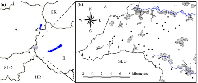
Study site

We conducted mycological surveys in Őrség National Park (ŐNP, 440 km²), West Hungary (46° 51′–55′ N, 16°

06′–24′ E (Fig. 1A). ŐNP is defined by the annual pre- cipitation range of 700–800 mm and situated at the bor- der of the subalpine and Pannonian climate zones. The mean annual temperature range is 9.1–9.8 °C, and the mean minimum and maximum temperatures are − 7.4 to 6.0 °C in winter and 13.5–23.8 °C in summer (Hungarian Meteorological Service). Nutrient-poor brown forest soils (planosols or luvisols) are the most frequent soil types (Halász et al. 2006) with a topsoil pH range of 4.0–4.8 (Juhász et al. 2011). ŐNP is a perfect place to examine the

effects of different tree taxa on forest-dwelling macrofungi due to its highly mixed forest stands with the dominance of beech (Fagus sylvatica), sessile and pedunculate oak (Quercus petraea and Q. robur), hornbeam (Carpinus betulus), and Scots pine (Pinus sylvestris) (Tímár et al.

2002). In our previous study (Kutszegi et al. 2015), we provided a comprehensive description of the region con- sidering its climate, soil characteristics, tree species and historical land uses.

Environmental data collection

To reduce the effects of edaphic heterogeneity on macrofungal species richness, we chose 35 mature, 70–100-year- old, monodominant, and mixed stands of beech, oak, Scots pine and hornbeam of varying proportions, which were located in relatively flat areas and not influenced directly by surface waters. Within each stand, we assigned a plot of 30 m × 30 m for macrofungal surveys (Fig. 1B). See Siller et al. (2013) for GPS coordinates of plots. The smallest distance among plots is 500 m to minimize the interfering effects of spatial autocorrelation. The plots cover a low elevation range (250–350 m a.s.l.) to reduce the effects of an underlying elevation gradient on fungal species richness.

We measured 67 potential environmental variables representing tree species composition, stand structure, soil and litter conditions, microclimate, landscape structure, and management history to test for relationships with macrofungal species richness (Table 1). Field measurements of environmental variables are detailed in Appendix A and in Kutszegi et al. (2015).

(a) (b)

N

S

W E

A

SLO

2 0 2 4 6 8 kilometers SLO

HR A

SK

H

Fig. 1 Borders of West Hungary; Őrség National Park is highlighted by gray (A). Geographical position of the 35 plots (coverage: 160 km²); vil- lages by gray (B). A: Austria, H: Hungary, HR: Croatia, SK: Slovakia, SLO: Slovenia

(4)

Table 1 Environmental variables tested for relationship with species richness of macrofungal functional groups and guilds

Abbreviation in Fig. 3 Environmental variable Unit Mean (range) Trans-

forma- tion Tree species composition

Beech Relative volume of beech % 27.9 (0.0–94.4) ln

Hornbeam Relative volume of hornbeam % 3.9 (0.0–21.8) ln

Oaks Relative volume of oaks % 36.4 (1.1–98.0) ln

Deciduous trees Relative volume of deciduous trees % 70.3 (21.7–100.0) ln

Pine Relative volume of Scots pine % 26.2 (0.0–76.9) ln

Conifers Relative volume of coniferous trees % 29.7 (0.0–78.3) ln

Non-dominant trees Relative volume of non-dominant trees % 0.02 (0.00–0.17) ln

Tree species richness Species richness of trees Number

of species/1600 m²

5.63 (2–10) ln

Tree diversity Shannon diversity of tree species – 0.847 (0.097–1.802) ln

Stand structure

Moss cover Cover of mosses m²/ha 247.4 (16.6–2201.6) ln

Herb cover Cover of understory vegetation m²/ha 740.8 (19.2–4829.3) ln

Shrub cover Cover of shrubs m²/ha 1052.8 (0.0–5616.1) –

Shrub density Density of shrubs and saplings (DBH = 0–5 cm) Stems/ha 952 (0–4706) ln

Tree density Density of trees (DBH > 5 cm) Stems/ha 593 (218–1393) –

Tree basal area Basal area of trees m²/ha 32.9 (21.5–42.3) –

Tree DBH Mean DBH of trees cm 26.6 (13.7–40.7) –

CV of tree DBH Coefficient of variation of DBH of trees (DBH > 5 cm) – 0.48 (0.17–0.98) –

Large trees Density of large (DBH > 50 cm) trees stems/ha 17 (0–56) ln

DW cover Total cover of dead wood including twigs m²/ha 261.6 (79.4–723.0) ln

Snag volume Volume of snags (d > 5 cm) m³/ha 8.99 (0.90–65.02) ln

Log volume Volume of logs (d > 5 cm) m³/ha 10.51 (0.17–59.48) ln

CWD volume Total volume of logs and snags (d > 10 cm) m³/ha 19.50 (1.93–73.37) ln

Beech DW Total volume of beech logs and snags (d > 5 cm) m³/ha 1.34 (0.00–12.07) ln Oak DW Total volume of logs and snags of oak species (d > 5 cm) m³/ha 3.36 (0.00–47.19) ln Deciduous DW Total volume of deciduous logs and snags (d > 5 cm) m³/ha 6.71 (0.24–56.46) ln Coniferous DW Total volume of coniferous logs and snags (d > 5 cm) m³/ha 6.05 (0.00–46.87) ln Decayed logs Relative volume of logs (d > 5 cm) in advanced (3–6) stages of

decay % 54.86 (8.25–98.61) –

Soil and litter

Soil cover Cover of bare soil m²/ha 146.7 (8.6–472.2) –

Soil pH pH of soil (in water)* – 4.33 (3.96–4.84) –

Hydrolytic acidity Hydrolytic acidity of soil (y1)* – 30.21 (20.68–45.22) –

Exchangeable acidity Exchangeable acidity of soil (y2)* – 15.27 (3.94–30.47) –

Soil C Carbon content of soil* % 6.45 (3.30–11.54) –

Soil K AL-extractable potassium content of soil* mg K₂O/100 g 7.74 (4.00–13.10) –

Soil N Nitrogen content of soil* % 0.22 (0.11–0.34) –

Soil P AL-extractable phosphorus content of soil* mg P₂O₅/100 g 4.29 (1.96–9.35) – Fine texture Fine texture (clay and silt) proportion of soil (2–63 μm fraction)* % 51.95 (27.60–68.60) –

Fine sand Proportion of fine sand (63–630 μm fraction)* % 38.16 (26.7–50.2) –

Coarse sand Proportion of coarse sand (0.63–2 mm fraction)* % 9.9 (1.5–45.7) ln

Litter cover Cover of litter m²/ha 9367 (7815–9834) –

Litter pH pH of litter (in water) – 5.29 (4.86–5.68) –

Litter C Carbon content of litter % 65.69 (42.87–78.09) –

Litter N Nitrogen content of litter % 1.28 (0.83–1.84) –

Litter mass Total litter mass (dried) g/900 cm² 147.7 (105.4–243.1) –

(5)

Fungal data

Due to the large total area (31,500 m²) of sampling units, we completed sporocarp surveys instead of DNA sequence-based identification techniques to characterize macrofungal species richness. We sampled basidiomycetes (excluding most of the resupinate non-poroid taxa) and ascomycetes that develop sporocarps larger than 2 mm.

We focused exclusively on species that belong to the main fungal functional groups: ECM, terricolous saprotrophic, and wood-inhabiting fungi (descriptions in Table S1). To sample the fungal species fruiting in spring, summer, or in autumn, we organized three sampling visits: in August 2009 (for 8 days), in May 2010 (8 days) and during Sep- tember–November 2010 (due to the perfect fruiting conditions, for 48 days). We fixed a species list in each plot, in each sampling visit, and merged the results of the three visits to obtain the total observed species richness of plots.

We detailed our species identification and nomenclatural

procedures in Kutszegi et al. (2015) and Siller et al.

(2013).

Statistical analysis

We divided our raw fungal species richness data into hierarchical subsets (guilds) based on the ecological functioning (F; 14 subsets) and host tree preference (H; 11 subsets) of fungal species (Fig. 2c, Tables S1, S2). Literature about the life strategy (functioning) of macrofungal species is mainly restricted to wood-inhabiting fungi; consequently, this classification is completed almost exclusively for this fungal group. The life strategy of several ECM and terricolous saprotrophic fungi is still unknown (Dighton 2003); therefore, we almost failed to separate guilds within them. Forming guilds, we classified the wood-inhabiting species according to their pathogenicity, type of rot, and life strategy following Pirttilä and Frank (2011) and Boddy et al. (2008).

*Soil layer: 0–10 cm, **radius = 300 m Table 1 (continued)

Abbreviation in Fig. 3 Environmental variable Unit Mean (range) Trans-

forma- tion

Decayed litter Mass proportion of decayed litter % 67.71 (51.58–84.16) –

Deciduous litter Mass proportion of deciduous litter % 14.71 (2.54–32.80) –

FWD in litter Mass proportion of fine (d < 5 cm) woody debris in litter % 11.9 (4.3–19.7) – Microclimate

Temperature Mean daily air temperature difference °C − 0.10 (− 0.93–0.73) –

Min. temperature Minimum daily air temperature difference °C − 0.50 (− 1.83–0.53) –

Max. temperature Maximum daily air temperature difference °C 0.44 (− 0.40–1.38) –

Temperature range Daily air temperature range difference °C 0.94 (− 0.42–2.49) –

Air humidity Mean daily air humidity difference % 0.84 (− 1.83–3.32) –

Min. air humidity Minimum daily air humidity difference % − 0.64 (− 5.72–3.21) –

Max. air humidity Maximum daily air humidity difference % 1.25 (− 0.44–3.47) ln

Air humidity range Daily air humidity range difference % 1.89 (− 2.27–6.58) –

Light Mean relative diffuse light % 2.93 (0.62–10.36) ln

CV of light Coefficient of variation of relative diffuse light % 0.51 (0.12–1.23) ln

Landscape

Renewals 300 Proportion of cutting areas** % 5.73 (0.00–23.03) ln

Forests 300 Proportion of forests** % 89.80 (56.92–100.00) –

Open areas 300 Proportion of open patches (settlements, meadows, arable lands)** % 8.57 (0.00–65.47) ln

Open areas 500 Proportion of open patches (radius = 500 m) % 4.72 (0.00–45.25) –

Old forests 500 Proportion of old-growth forests (radius = 500 m) % 85.77 (37.48–98.48) – Landscape diversity 300 Shannon diversity of landscape elements** – 1.114 (0.108–1.858) – Management history

Historical forests Proportion of forests in 1853** % 76.58 (24.03–100.00) –

Historical meadows Proportion of meadows in 1853** % 7.26 (0.00–40.73) –

Historical arable lands Proportion of arable lands in 1853** % 16.16 (0.00–61.27) –

Locality of forests Locality of forests in 1853 Binary 0.80 (0–1) –

Locality of arable lands Locality of arable lands in 1853 Binary 0.17 (0–1) –

(6)

For the exploration of the relationships between species richness data and environmental variables, we built multiple regression models, applied general linear modeling (GLM) based on Faraway (2005, 2006), and used the statistical soft- ware R for Windows 3.0.1 (R Core Team 2013).

Prior to building GLMs:

(a) We checked the normality of each potential explanatory and response variables. Some explanatory variables were needed to be ln-transformed to satisfy the criterion of normality (Table 1). For the response variables (Table S1), no logarithmic transformations were needed.

(b) We centered and standardized the explanatory variables by standard deviation.

(c) We corrected each of our response variables for sampling bias because our field survey in autumn lasted for 48 days until the end of (or beyond) the fruiting period of some fungal species. We numbered the days of this sampling period from 1 to 48 to create a “sampling time” variable and then applied partial correlations according to Legendre and Legendre (1998) to remove (partial out) the distorting effects of sampling bias.

(d) We screened the explanatory variables for collinearity. First, calculating correlation matrices, we com-

pleted correlations pairwise between each response and each potential explanatory variable to select the explanatory variables with a homogeneous relationship stronger than |r| = 0.35 to a response variable. Among these explanatory variables, we screened the ones with a stronger collinearity of |r| > 0.45 and excluded the variable(s) with a weaker effect to the response variable.

Due to the under-dispersion of variances, pinpointed by the R package “AER” (Kleiber and Zeileis 2008), we fit- ted quasi-Poisson GLMs to our species data following Zuur et al. (2009). We applied a manual backward selection for the full models by dropping the explanatory variables step- wise until all the remaining variables met the criterion of p < 0.05 within the models (based on deviance analyses with F-statistics). We calculated a pseudo-R² to our quasi-Poisson GLMs based on McFadden (1974), and applied deviance analyses with F-statistics to establish a statistical reliability for the final models. For each final model, we checked the validation graphs to assess the homogeneity and normality of residuals, homoscedasticity, and Cook statistics to reveal whether any observation has extreme values of the explanatory variables. Finally, using the R package “faraway”

(Faraway 2002), we calculated a variance inflation factor

Models built on terricolous saprotrophic fungi (n = 5) ...on ECM fungi (n = 3) ...on wood-inhabiting fungi (n = 14) ...on functional groups (models F1–F14) ...on groups by host tree preference (H1–H11)

F1 F2 F3 – 2 F4 F5 F6 F7 F8 F10 F11 F12 F14 – 3 F13 F9 – 4 FULL SAMPLE classification level 1

H1 H2 H3 – 2 H4 H5 H6 H7 H8 H9 H10 H11 – 3 Division by

functional groups

...by host tree preference

(a)

(b) (c)

0.3 0.4 0.5 0.6 0.7

R² FULL SAMPLE – 1

Fig. 2 Comparison of R²-values of 26 quasi-Poisson linear models shown in Fig. 3; grouping of models by main functional groups (a), division methods (b), and classification levels within divisions (c). Part (c) details briefly the hierarchical arrangement of models.

We detected slight dissimilarities but no evidences of significant (p < 0.01) differences among R²-values. We performed ANOVA and Student’s t tests to complete multiple (a, c) and paired (b, c) com- parisons, respectively (see text for p values). ECM fungi had con-

sequently lower R²-values (a). Models on subsets separated based on fungal host tree preferences were stronger because we included explanatory variables that characterize the species composition of trees (b). Probably due to concordant species responses, models done on functional groups and on species groups by host tree preference tended to be a bit stronger toward lower classification levels (c).

Box metrics: central line, median; box, inter-quartile range; whisker, 1.5 × inter-quartile range

(7)

(Faraway 2005) for each explanatory variable included in the final models to screen them for multicollinearity.

Applying ANOVA or Student’s t test, we compared the R² values of models done on the subsets of (i) the three main functional groups, (ii) our two groups of models (subsets by ecological functioning vs. host tree preference), and (iii) the classification levels within the two model groups of point (ii). To help understand the drivers of the three main functional groups, we classified the drivers of their subsets based on their significance and the number of subsets they form. By this simultaneous evaluation of models, we got the possibility to highlight those drivers of subsets that (i) cannot be detected by the exclusive modeling of the main functional groups and (ii) possibly have indirect effects on the main functional groups.

Results

Macrofungal diversity

We observed 676 fungal taxa (Table S2), obtaining 4067 records. Of these, we collected 896, 274, and 2897 records in August 2009, in May 2010, and during autumn 2010, respectively.

Different guilds, different drivers: substrate and host were decisive

We separated and modeled 25 subsets of the full sample (Fig. 3); hierarchical arrangements of subsets are in Fig. 2c, more statistical details of models in Figs. S1 and S2.

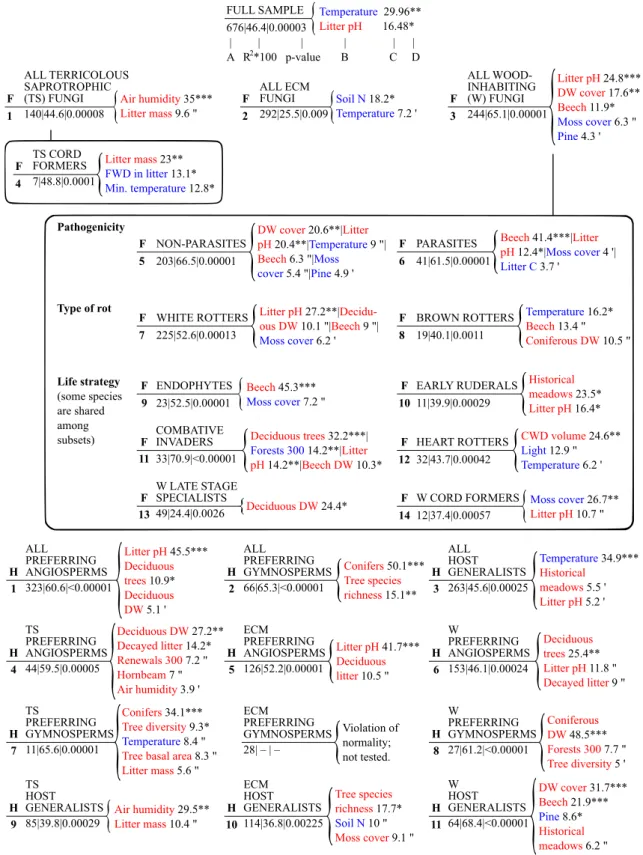
The environmental variables revealed by all of our models can be arranged into our six variable groups with the following proportions: soil and litter conditions (28%; 23 significant variables out of the 80 revealed in total), tree species composition (25%), stand structure (24%), microclimate (15%), landscape structure (4%), and management history (4%). In general, the three main functional groups (models F1–F3) and other large subsets with more than 200 modeled species (F5, F7) were driven principally by the general environmental requirements of macrofungi: microclimate (temperature) and substrate properties (pH of litter, soil nitrogen content, and amount of dead wood). By contrast, the small subsets of 7–49 species were mainly formed by more specific drivers representing the stand structure, the chemical components of the soil and litter layer, and the surrounding landscape.

Specifically, the species richness of terricolous saprotrophic fungi (F1) was driven by air humidity and litter mass.

ECM fungi (F2) were negatively determined by the nitrogen content of soil and air temperature. Wood-inhabiting

macrofungal species richness (F3) was principally formed by litter pH, dead wood cover, and beech proportion.

Wood-inhabiting fungal guilds (F5–F14) were mainly determined by well-interpretable drivers not detected at the level of all wood-inhabiting fungi. However, two drivers (litter pH and beech proportion) influenced both the group of all wood-inhabiting fungi and some of its subsets, but usually with highly different importance. Non-parasites (F5) were principally shaped by total dead wood cover and litter pH, whereas beech proportion was the most important driver for parasites (F6). White rotters (F7) were found to be a substrate-related guild following stands with high litter pH and high proportion of deciduous dead wood. By contrast, brown rotters (F8) were mainly driven by microclimate (air temperature, negatively), while the effects of host (beech) and substrate (total volume of coniferous logs and snags) were less pronounced. Wood-inhabiting fungal guilds defined by life strategies (F9–F14) and describing consecutive stages of wood decay were determined by drivers different from each other. Endophytes, with the ability to switch from a biotrophic to a saprotrophic lifestyle, favored stands with high beech proportion. Early ruderals, colonizing freshly exposed dead wood units, preferred forest stands that were formerly meadows and had a relatively high litter pH. Combative invaders were selective to stands with a high total proportion of deciduous tree taxa, less surrounded by forests, and with higher litter pH. Heart rotters responded significantly to higher CWD volumes. Late stage specialists were determined exclusively by the total volume of deciduous logs and snags. Wood-inhabiting cord formers avoided stands with a high moss cover on the forest floor.

Terricolous saprotrophic cord formers (F4) were positively affected by litter mass, while FWD mass proportion and minimum air temperature had negative effects.

Guilds formed by host tree preference (H1–H11), expect- edly, responded most significantly to variables describing tree species composition (deciduous vs. coniferous). How- ever, the other drivers within the models carry valuable information. All the models on fungal species selective for coniferous habitats (H2, H7, and H8) pointed out a specific requirement of higher host tree diversity in conifer-dominated stands. Host generalists (H3, H9–H11) responded to similar drivers, but with different importance as that of the full sample and the main functional groups (F1–F3). Con- trasting model F1 with H9 about terricolous saprotrophic fungi, the two models revealed the same results: high air humidity and high litter mass were needed. Host generalist ECM fungi (H10) mainly required higher tree species richness with higher moss cover; the low soil nitrogen content had only marginal effects. By contrast, all ECM fungi (F2) were primarily shaped by soil nitrogen content. Host generalist wood-inhabiting fungi (H11) were determined by dead wood cover followed by more beech and less Scots pine,

(8)

FULL SAMPLE 676|46.4|0.00003

Temperature 29.96**

Litter pH 16.48*

Litter mass 23**

FWD in litter 13.1*

Min. temperature 12.8*

TS CORD FORMERS 7|48.8|0.0001

{

F 4

Conifers 50.1***

Tree species richness 15.1**

ALLPREFERRING GYMNOSPERMS 66|65.3|<0.00001 H

2

{

Temperature 34.9***

Historical meadows5.5 ' Litter pH 5.2 ' ALLHOST

GENERALISTS 263|45.6|0.00025 H

3

{

Litter pH 45.5***

Deciduous trees 10.9*

Deciduous DW 5.1 ' ALLPREFERRING

ANGIOSPERMS 323|60.6|<0.00001 H

1

Air humidity 35***

Litter mass 9.6 "

ALL TERRICOLOUS SAPROTROPHIC (TS) FUNGI 140|44.6|0.00008

{

F 1

Soil N 18.2*

Temperature 7.2 ' ALL ECM

FUNGI 292|25.5|0.009

{

F 2

ALL WOOD- INHABITING (W) FUNGI 244|65.1|0.00001 F

3

Litter pH 24.8***

DW cover 17.6**

Beech 11.9*

Moss cover 6.3 "

Pine 4.3 '

{

Pathogenicity DW cover 20.6**|Litter pH20.4**|Temperature 9 "|

Beech 6.3 "|Moss cover5.4 "|Pine 4.9 ' NON-PARASITES

203|66.5|0.00001

{

F 5

Beech 41.4***|Litter pH12.4*|Moss cover 4 '|

Litter C 3.7 ' PARASITES

41|61.5|0.00001

{

F 6

Type of rot Litter pH 27.2**|Decidu- ous DW 10.1 "|Beech 9 "|

Moss cover 6.2 ' WHITE ROTTERS

225|52.6|0.00013

{

F 7

Temperature 16.2*

Beech 13.4 "

Coniferous DW 10.5 "

BROWN ROTTERS 19|40.1|0.0011

{

F 8

Life strategy (some species are shared among subsets)

Moss cover 26.7**

Litter pH 10.7 "

W CORD FORMERS 12|37.4|0.00057

{

F 14 Deciduous trees 32.2***|

Forests 300 14.2**|Litter pH14.2**|Beech DW 10.3*

COMBATIVE INVADERS 33|70.9|<0.00001 F

11

{

Deciduous DW 24.4*

W LATE STAGE SPECIALISTS 49|24.4|0.0026 F

13

{

CWD volume 24.6**

Light 12.9 "

Temperature 6.2 ' HEART ROTTERS

32|43.7|0.00042

{

F 12 Beech 45.3***

Moss cover 7.2 "

ENDOPHYTES 23|52.5|0.00001

{

F 9

EARLY RUDERALS 11|39.9|0.00029 F

10

Historical meadows 23.5*

Litter pH 16.4*

{

Deciduous DW 27.2**

Decayed litter 14.2*

Renewals 300 7.2 "

Hornbeam 7 "

Air humidity 3.9 ' TSPREFERRING

ANGIOSPERMS 44|59.5|0.00005 H

4

Conifers 34.1***

Tree diversity 9.3*

Temperature 8.4 "

Tree basal area 8.3 "

Litter mass 5.6 "

TSPREFERRING GYMNOSPERMS 11|65.6|0.00001 H

7

Air humidity 29.5**

Litter mass 10.4 "

TSHOST GENERALISTS 85|39.8|0.00029 H

9

{

Litter pH 41.7***

Deciduous litter 10.5 "

ECMPREFERRING ANGIOSPERMS 126|52.2|0.00001 H

5

{

Tree species richness 17.7*

Soil N 10 "

Moss cover9.1 "

ECMHOST GENERALISTS 114|36.8|0.00225 H

10

Deciduous trees 25.4**

Litter pH 11.8 "

Decayed litter 9 "

WPREFERRING ANGIOSPERMS 153|46.1|0.00024 H

6

{

Coniferous DW 48.5***

Forests 300 7.7 "

Tree diversity 5 ' WPREFERRING

GYMNOSPERMS 27|61.2|<0.00001 H

8

{

DW cover 31.7***

Beech21.9***

Pine 8.6*

Historical meadows 6.2 "

WHOST GENERALISTS 64|68.4|<0.00001 H

11 Violation of normality;

not tested.

ECMPREFERRING GYMNOSPERMS

28| – | –

{

Fig. 3 Species richness models (quasi-Poisson GLMs) on the environmental drivers of macrofungal functional groups. To reveal the drivers cannot be detected by the exclusive test of the full sample, we divided the full sample based on the ecological function (F1–

F14) and host tree preference (H1–H11) of fungal species and built a separate model on each subset (guild). The simultaneous exami- nation of the drivers of subsets helps understand the drivers of the

main (F1–F3) functional groups. A: total number of modeled taxa, B:

drivers with negative (blue) and positive (red) effects, C: percent proportion of variance explained, D: significance codes: *** < 0.0001;

** < 0.001; * < 0.01; (″) < 0.05; (′) < 0.1. Serial numbers of models in bold; response variables by capital letters. Hierarchical arrangements of subsets are in Fig. 2c; more statistical details in Figs. S1 and S2

(9)

whereas all wood-inhabiting fungi (F3) responded primarily to litter pH and only secondarily to dead wood cover and beech proportion.

Indirect effects

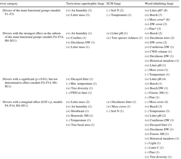
We classified the drivers revealed by the GLMs in Fig. 3 to separate the most important (determinative) ones from those of with marginal or probable indirect effects (Table 2).

Checking the drivers for common occurrences in the same models, we marked (asterisk) three drivers in category A to have probable indirect effects on macrofungi in the region.

All wood-inhabiting fungi (F3) were most significantly driven by litter pH. To try to explain this unexpected result, we compared the drivers of all the 11 subsets that were significantly formed by litter pH. In eight out of 11 cases (F3, F5–F7, F11, H1, H5, and H6), we observed that litter pH was selected together with drivers characterizing deciduous

Table 2 Classification of drivers revealed by the GLMs in Fig. 3 forming terricolous saprotrophic, ECM, and wood-inhabiting macrofungal species richness

Categories are assigned based on the significance of drivers; the numbers, in brackets, show the number of models in which the drivers were included. Drivers in category “A” were detected several times forming the subsets of the main functional groups; therefore, they may have true determinative effects on macrofungi in the region. Category “B” and “C” list the most important drivers of subsets that affect in a hidden way when the main functional groups are exclusively studied. Often with probable indirect, hardly interpretable effects, drivers in category “D”

should be viewed with an extra caution. Drivers with an asterisk may affect indirectly (details in the text). Concerning the direction of effects, drivers were affected consistently within functional groups

Driver category Terricolous saprotrophic fungi ECM fungi Wood-inhabiting fungi

A Drivers of the main functional groups (models

F1–F3) (+) Air humidity (3) (–) Soil N (2) (+) Litter pH* (8)

(+) Litter mass (3) (–) Temperature (1) (+) Beech (7) (–) Moss cover* (6) (+) DW cover (3) (–) Pine* (3) B Drivers with the strongest effect on the subsets

of the main functional groups (models F4–F14, H4–H11)

(+) Air humidity (1) (+) Litter pH (1) (+) Beech (2) (+) Conifers (1) (+) Tree species richness (1) (+) Deciduous trees (2)

(+) Deciduous DW (1) (+) DW cover (2)

(+) Litter mass (1) (+) Coniferous DW (1)

(+) CWD volume (1) (+) Deciduous DW (1) (+) Historical meadows (1) (+) Litter pH (1)

(–) Moss cover (1) (–) Temperature (1) C Drivers with a significant (p < 0.01), but not

determinative effect (models F4–F14, H4–

H11)

(+) Decayed litter (1) (+) Litter pH (4)

(–) Min. temperature (1) (+) Beech (1)

(+) Tree diversity (1) (+) Beech DW (1)

(–) FWD in litter (1) (–) Forests 300 (1)

(–) Pine (1) D Drivers with a marginal effect (0.05 < p; models

F4–F14, H4–H11) (+) Litter mass (2) (+) Deciduous litter (1) (–) Moss cover (4)

(+) Air humidity (1) (+) Moss cover (1) (+) Beech (3)

(+) Hornbeam (1) (–) Soil N (1) (–) Temperature (3)

(+) Renewals 300 (1) (+) Litter pH (2)

(–) Temperature (1) (+) Coniferous DW (1)

(+) Tree basal area (1) (+) Decayed litter (1)

(+) Deciduous DW (1) (+) Forests 300 (1) (+) Historical meadows (1) (–) Light (1)

(–) Litter C (1) (–) Pine (1) (+) Tree diversity (1)

(10)

habitats. In addition, model H1, about all fungal species selective for deciduous habitats, emphasized litter pH with the strongest effect.

Despite the fact that we checked our explanatory variables for collinearity within the models, we did find some cases when two drivers repeatedly co-occurred in the same model. For example, moss cover was very likely to co-occur with beech proportion; see model F3, F5–F7, and F14 (in 5 models out of 7). Also, Scots pine proportion showed the same pattern with beech in all models in which it was significant (F3, F5, and H11).

Comparison of the explanatory powers of models We compared the R²-values of our GLMs and found slight, non-significant differences (Fig. 2): among the main functional groups (ANOVA, p = 0.2679, a), division methods (Student’s t test, p = 0.2267, b), and among classification levels within division methods (for functional groups, ANOVA, p = 0.519; for host tree preference, Student’s t test, p = 0.6703, c).

Discussion

Drivers of macrofungal functional groups and guilds The species richness of macrofungal communities in the ŐNP was mainly formed by drivers describing soil and litter conditions, tree species composition, and stand structure (in this order). Microclimate, landscape structure, and management history had minor effects. Similar results have long been reported by several authors (Daws et al. 2020; Krah et al. 2018; Boddy et al. 2008; Smith and Read 2008; Ker- naghan et al. 2003) concluding that macrofungi, in general, are primarily substrate and host-restricted organisms.

Terricolous saprotrophic fungi were positively determined by air humidity and litter mass. McMullan-Fisher et al. (2009) did not directly measure air humidity but found that a higher annual rainfall and air temperature are important for all macrofungi in various (in both dry and humid) Eucalyptus forests of Tasmania. Tyler (1991) revealed that the experimentally doubled amount of litter enhances the sporocarp production of soil saprotrophs which is in line with our results. It is interesting that, in our study, microclimate had stronger effects on terricolous saprotrophs, which are thought to be a principally substrate-restricted organism group in temperate forests (Boddy et al. 2008).

ECM fungi were negatively driven by soil nitrogen content and air temperature. This result is concomitant with the results of other authors, e.g., Cox et al. (2010) and Peter et al. (2001) who have reported that the high soil nitrogen content has generally negative effects on the fruiting of

several ECM fungal species in temperate forests. However, the opposite was also confirmed in severely nitrogen-limited boreal forests (Perez-Moreno and Read 2001). In our study, the general preference of ECM fungal species to lower air temperatures cannot be explained clearly based on the drivers of our guilds. The phenomenon may be clarified by the fact that the studied region is a home to many ice age relic ECM fungal species with boreal distribution centers, for which the area is a refuge; see Siller et al. (2013) and Vasas and Locsmándi (1995) for species lists. Several boreal ECM species are selective to lower temperatures (Smith and Read 2008).

Wood-inhabiting fungi, surprisingly, was determined by litter pH. Dead wood cover and beech proportion were less significant, while the total moss cover (together on soil and dead wood units) and Scots pine proportion had marginal (and probably indirect) effects. To our knowledge, litter pH also has indirect effects on wood saprotrophs and highlights a general preference of deciduous habitats (detailed in the next chapter). It can be explained by the fact that most (92%) of our collected wood saprotrophs was a white rotter, generally preferring angiosperm wood (Krah et al. 2018), and two-third of all (63%) were exactly selective to deciduous trees. Wood-inhabiting fungi are substrate-restricted organisms (Boddy et al. 2008); thus, their high dependence on available dead wood is obvious and was repeatedly reported by many authors: Heilmann-Clausen et al. (2014), Stok- land et al. (2012), and Kirk and Cowling (1984). The strong effect of beech in our study on wood-inhabiting fungi can be explained by both the quick production of large dead wood volumes in the fast-growing beech stands (Heine et al. 2019) and the relatively high cellulose content of beech wood (Schwarze and Baum 2000). Beech forests were mentioned among the richest habitats in wood saprotrophs (Küffer and Senn-Irlet 2005); and according to Heine et al. (2019), beech specifically promotes the diversity and species richness of wood-inhabiting fungi in Europe.

Cord-forming litter saprotrophs were enhanced by litter mass and suppressed by fine woody debris proportion.

Litter is the main substrate of this guild which was well- illustrated by Boddy et al. (2009) demonstrating that cord formers mainly grow at the soil–litter interface intercon- necting and consuming litter components. Large amounts of FWD in litter may inhibit hyphal growth by facilitating the aeration and slowing the compaction of the lower litter layer making the environment less favorable for fungi (Berg and McClaugherty 2014).

Non-parasitic and parasitic (necrotrophic) wood-inhabiting fungi showed highly differing requirements. Most species were shared between non-parasites and all wood- inhabiting fungi; therefore, both groups were shaped by similar drivers with fine differences in importance. By contrast, necrotrophic parasites were clearly determined

(11)

by beech proportion. According to Schwarze et al. (2000), beech harbors a relatively rich community of parasitic fungi in Central European temperate forests. This phenomenon is not completely understood but can be explained by the wide geographical distribution, large body size, fast growth, and thin, vulnerable bark (Biggs 1992) of beech, as well as its high cellulose and low lignin and tannin contents (Schwarze and Baum 2000). In our data set, half of the tree parasites indeed preferred beech as a primary host.

White rotters and brown rotters differed strongly in their drivers. We mainly found white rotters in deciduous habitats, which is in accord with the strong, positive effects of litter pH, deciduous dead wood, and beech proportion in their model. Their requirements were very similar to those revealed for all wood-inhabiting fungi. They were found to be substrate-restricted. Based on the phylogeny of more than 1000 wood-inhabiting fungal species from the North- ern Hemisphere, Krah et al. (2018) found that most white rot fungi are angiosperm specialists owing to the closely simultaneous diversification of these fungal group and angiosperms in the Cretaceous. In contrast, brown rotters were primarily suppressed by high air temperatures and enhanced by high amounts of coniferous dead wood. We failed to join this temperature relation to previous studies, but we attempt to explain the phenomenon with the generally cooler microclimate of coniferous stands compared to that of deciduous ones. Heat loss is generally higher in coniferous stands where the canopy openness is high due to the narrow leaves.

According to Krah et al. (2018) and Hibbett and Donoghue (2001), most brown rot fungi are gymnosperm specialists supposedly because their lineages originated during the diversification of gymnosperms.

Similar to parasitic wood-inhabiting fungi, endophytes were linked strongly to high beech proportion. This is con- sistent with the results of Unterseher and Schnittler (2010) and Sieber (2007) who mentioned beech as one of the most species rich host for endophytes and other wood saprotrophs (Heine et al. 2019) in Central European forests. Here, beech plays a similar role in the ŐNP significantly forming the species richness of several subsets. The chemical and struc- tural characteristics of beech wood are detailed above for parasites; these properties probably also explain the strong effects of beech on endophytes.

Early ruderals were driven primarily by forest management history; they responded to the high proportion of meadows surrounding the sampling unit c.a. 160 years ago. Cau- tion must be used in interpretation of this result because their model has little explanatory power and a very low number of tested species. Moreover, all of our sampling units were assigned in stands older than 70 years which is enough time for some dead wood to be produced and many early ruderals (even some late stage specialists) to establish (Boddy and Heilmann-Clausen 2008; Boddy 2001). Once some

dead wood is produced, the habitat is open for decomposer fungi; therefore, it is unimaginable that a variable expressing a 160-year-old situation could significantly affect this group.

Combative invaders were determined by the high proportion of deciduous trees and substrates. These combative secondary colonizers can cause rapid white rot on fallen logs and branches (Boddy and Heilmann-Clausen 2008) domi- nating the decomposition of angiosperm wood (Hibbett and Donoghue 2001). Interestingly, they were negatively affected by the proportion of forests in the landscape which can be likely explained by the general low amount of dead wood in the surrounding old stands close to their age of harvest.

Following silvicultural activities, cutting areas are opened and some substrates (mainly stamps) can be produced for these fungi.

Heart-rot agents responded significantly to CWD volume.

This is in accord with the conclusions of Moore et al. (2008) about the relatively high nitrogen requirement of heart rotters among wood decay fungi. To acquire enough nitrogen for the development of big, perennial sporocarps, heart rotters must establish large mycelial domains and colonize large dying trees and dead wood units.

The species richness of late stage specialists was significantly higher in stands with high amounts of deciduous dead wood. Surprisingly, the proportion of decayed logs had no detectable effects probably due to the general low amounts of this substrate in our sampling units. Toward the final stage of wood decomposition, Renvall (1995) found an increasing number of white rotters at the expense of brown rotters because white rotters have enzymes to degrade the more complex wood components (lignin and hemicellulose), in which the well decayed dead wood units are generally richer.

Wood-inhabiting cord formers were negatively influenced by moss cover. It is known that soil respiration and decomposition rates can be significantly reduced by a well- developed moss layer (Nilsson and Wardle 2005). Study- ing Armillaria mellea rhizomorphs growing in deeper soil layers, Morrison (1976) reported decreasing oxygen and increasing carbon-dioxide levels to have limiting effects on rhizomorph growth and wood decomposition. Modeling the species composition of all wood-inhabiting fungi on logs of deciduous trees, Ruokolainen et al. (2018) and Heilmann- Clausen et al. (2005) also observed moss cover with significant effects and concluded that it may have stabilizing effects on the microclimatic environment within the wood and can cause shifts in the species composition rather than in the species richness of wood-inhabiting fungi.

Drivers affecting indirectly

The group of all wood-inhabiting fungi was primarily determined by litter pH. To our knowledge, litter pH has never been detected as a driver of this functional group. Here, in 8

(12)

models of 11, litter pH was significant and selected together with drivers characterizing deciduous habitats. This provides some evidence that litter pH rather represents a general preference of deciduous habitats not the special impacts of litter pH per se. Another variable of probable indirect effects on wood-inhabiting fungi was moss cover, always with sup- pressing effects and acting as a follower of beech proportion (in 5 models out of 7). Working in shaded, beech-dominated habitats with a generally poor moss layer, Heilmann-Clausen and Christensen (2005) also confirmed this observation.

Similarly, Scots pine proportion was always co-acted with beech proportion and rather had marginal effects on wood- inhabiting fungi. We found no drivers with probable indirect effects for terricolous saprotrophic and ECM fungi.

The importance of tree diversity and tree species richness was specifically revealed in coniferous habitats exclusively forming those guilds that species were selective for coniferous hosts. Conifer-dominated forests harbor a distinc- tive mycota with species of specific abilities to decompose needle litter and coniferous wood (Humphrey et al. 2000).

In such habitats, increasing tree diversity by broadleaved tree species can make major contributions to a richer fungal community.

Is it worth modeling fungal guilds?

Former studies on environmental drivers have mainly focused on all the wood-inhabiting (e.g., Krah et al. 2018;

Ruokolainen et al. 2018; Abrego and Salcedo 2013), ECM (e.g., Van Nuland and Peay 2020; Cox et al. 2010; Smith and Read 2008), or terricolous saprotrophic fungi (e.g., Reverchon et al. 2010; Boddy et al. 2009; McMullan-Fisher et al. 2009) in the studied region. Within these groups, guilds have rarely been formed and modeled (but see Štursová et al.

2020; Heilmann-Clausen et al. 2014, and Boddy 2001) due to the limited knowledge on the life strategies, substrate preferences, and environmental requirements of several fungal species (Dighton 2003). Working with guilds is difficult because many fungal species can switch among life strategies along changing environmental conditions (Zanne et al. 2020). Hence, it is impossible to establish discrete boundaries among them (Pirttilä and Frank 2011). Moreo- ver, numerous different grouping methods can be applied onto the same species pool. Guilds can be defined as community components with similar effects on, or with concordant responses to the environment (Hooper et al. 2002).

Guilds can also be defined as groups of species competing for the same resources, inhabiting a certain microhabitat, or community components exploiting different resources but in related ways (Simberloff and Dayan 1991). Here, we also set up guilds based on different point of views. We tried to overcome the aforementioned problems by constructing guilds according to criteria that are related fundamentally

to the general environmental drivers of macrofungi, representing substrate quality and quantity, life history, and host tree taxonomy. In whatever aspects we formed guilds, we often got groups with less than 40 species, for which we also obtained models with strong (R² × 100 > 50) explanatory powers. Moreover, for many guilds, we usually revealed drivers that were not detected (were hidden) modeling the entire functional group containing the guild.

Proofs of concordant species response

A species richness model will be strong when: (i) the tested species group actually forms a guild with concordant species responses to the environment, (ii) exactly those environmental variables were measured that are truly important for the species group, and (iii) the model contains several (3–5) significant variables. The positive effect of concordant species response on the explanatory power of models can also be observed in our results: models done on host generalists often detected weaker responses compared to the models on host specialists.

Our generally weaker models on ECM fungi can be explained by the following reasons: (i) we probably did not measure those environmental variables that really influence these species in the region, (ii) it is not yet clear which of these species form a guild and have similar environmental requirements, and (iii) it is highly probable that our model on all ECM fungi contains several guilds (species) that are driven principally by different environmental drivers.

Deveautour et al. (2020) also suggested numerous guilds within ECM communities. It would be especially worth- while for ECM fungi to find the environmental requirements of single species using linear regression models. With such models, we could define ECM guilds that consist of species with similar responses to the environment and thus better understand the functioning of the whole ECM community.

Our model on all litter saprotrophs was weaker than the model on cord-forming litter saprotrophs. Due to this, several embedded litter saprotrophic guilds can be suggested within the main functional group of litter saprotrophs. Long- term studying litter decomposition, Štursová et al. (2020) revealed consecutive successional phases along the breakdown process to be dominated by different litter saprotrophic fungal guilds.

Limitations

We exclusively sampled sporocarps for a short duration (2 yrs) of field visits to measure macrofungal species richness.

It is an underestimate of the total species richness in the studied region because we consistently skipped to register microfungi (those that never produce sporocarps) and cer- tainly have overlooked some of those macrofungal taxa that