COMPUTER AND AUTOMATION INSTITUTE, HUNGARIAN ACADEMY OF SCIENCES
MULTI ELEMENT FAULT ISOLATION IN ELECTRONIC CIRCUITS
N.N.PURI
Prof, of Electrical Engineering, Rutgers University,
New Brunswick, New Jersey,USA
Reports 54/1976
Responsible Publisher T. Vámos
Készült az Országos Műszaki Könyvtár és Dokumentációs Központ házi sokszorosítójában
F.v.: Janoch Gyula
3
ABSTRACT
A method is developed for the identification of the each of the faulty elements in the linear Electronic Circuits when one or more of the elements are simultaneously off from their nominal value. Exact analytical expressions are presented for the
identification of one and two simultaneously faulty elements, along with the algorithm for the multiple faulty elements case.
m _
In general for an m element fault, 2 different measurements are made (real and imaginary part). These measurements may
III" 1
involve transfer function frequency response at 2 different frequencies, or in case of degeneracy, different functions such as input inpedances, etc. , such that total different
measurements are 2m ^ . Method is discussed by means of examples.
liaWÄS
.
1. INTRODUCTION
A method of fault isolation in the linear circuits for a single faulty element has been proposed by Martens and Dyck c II and others1"211 11 ^2 using bilinear transformation. The method is graphical in nature, producing frequency domain loci which depend upon the value of the assumed faulty element. The
faulty element is identified by the location of the test meas
urements of the equipment on a particular loci. Besides having the limitation of being applicable to a single element fault only, the method is cumbersome for automatic computer mecha
nization. In this paper we present analytical expression for the identification of one or two faulty elements and derive a general algorithm for the multi elements fault case. We shall assume that the symbolic transfer dunctions (or different transfer functions between different sets of terminals) is k n o w n 1" ^ The method of fault identification is explained by means of examples.
2. PROBLEM STATEMENT AND ASSUMPTIONS
The problem proposed consists in isolating faulty elements (one or more) in a lumped, linear time invariant, active elec
tronic networks. It is assumed that the topology of the
network and the nominal va l u e of the components are known, so that the symbolic transfer function can be obtained. It is futher assumed that failures are not catastrophic and enough test terminals are available to obtain frequency response which is dependent on the value of elements which are faulty.
3. METHOD OF SOLUTION 3.1 Single faulty element
Let the various elements such as transistors, resistors
etc. of the network be symbolized by p^, p 2 ,...,p , n being the total number of elements. The nominal value of these ele
ments be given by p 1 Q , P 2o r**,'Pno*
Let
0 < --- = x., P i i=l,...,n 3.1.1 p 10 1
When all x.^, (i=l,...,n) are unity, the equipments is not faulty.
Let us consider the situation when a particular kth compo
nent is faulty, such that x ^ ^ 1. Problem reduces to determining all different x's and thus the faulty element and its value.
The system transfer function T(s) can be written in n dif
ferent forms1:7:1 as
- 6 -
A,(s) x + B, ( s )
T(s) = T(s,xk ) = c (s ) x + D. (s )* (k=l,...,n) 3.1.2
Let us obtain the frequency of this equipment at one particu
lar frequency w, involving phase and amplitude measurement and hence the real R(üj) and imaginary part X(w), yielding
T ( jtu) = R(iu) + jx(u)
Ak (jw) xk + Bk (jw)
ck (jw) xk + Dk (ju) (k=l ,n) 3.1.3
The test frequency is choosen with regard to the nominal poles C 8 Cl
and zeros locations, as discussed by Seshu and Waxman Let
A k (jw) = A k (w) + jAk (w)
1 2
Bk (jw) = Bk l (w) + ^Bk 2 ^w ^ Ck (jw) = c U ) + jck ^(m) Dk (jo>) = Dk ( u ) + j D k ( w )
1 2
3.1.4
7
Substituting 3.1.4 into 3.1.3 and equating real and imaginary p a r t ,
(R(w)C, (to )-X( to )C (to))x + (R(w)D (to)-X(to)D ( to) )
K2 -K* K ^
= Ak (a))xk + Bk (to)
3.1.5 (R(u)C, (to) + X(to) C (to))x + (R(to)D (to) + X(to)D, (to))
= A, (<o)x + B (to)
k 2 K K2
The relations 3.1.5 are true only when k 1' element symbolized th by x, is the faulty element. The quantities A. (to) etc. are
K K
computed for the nominal values of other elements (except of course the k tk element). Since both the equations of 3.1.5 should give the same value of xk , the condition that k th element is indeed the faulty one is given by eliminating xk from equations 3.1.5 to yield.
( X2 ( ü) )+R2 (to) ) ( C. (w)D, (to)-C, (to) D. ( a>) ) + k l' ” k 2 k2 k l
+ R( i o ) ( D, (to)A, ( to )+C, (to)B ( t o ) - D (to)A ( t o ) - C (to)B ( a)) )
K 1 k 2 K 2 K 1 K 2 1 1 2
+ X ( w ) ( C , (to)B ( to)+C ( u ) B ( <o) - D (to)A ( t o ) - D (to)A ( t o ) )
K 1 K 1 k 2 K 2 K 1 K 1 K 2 2
+ (Ak (w)Bk (to)-Ak (to)Bk (to) = Ak (to) = 0 3.1.6
Theoretically only frequency measurement at one frequency is necessary, but due to noise consideration, the condition
3.1.6 may be verified at different frequencies. If 1 m ~
Í z A k (a)i } m i=1 k 1
is less than some precomputed number £, then the condition
3.1.6 is considered fulfilled. Furthermore value of x, should k
be positive.
- 8 -
3.2 Example
Consider simple circuit given in Figure 3.2.1
Let the nominal values of these various elements be
R1
llc1—«II lOOO Kft
c II
11ouii 1 yF = i o- 6f 3 . 2 . 1
R2 = R2 0 = 3 0 0 0 KÍ2
The actual values of these elements are cy response
u~( s)
at u)=l is
such that the frequen-
R ( w )
X ( w )
11 26
_3 26
3 . 2 . 2
Only one element is considered off from the nominal value. We are required to find this element and its value.
Let
x1' 3 . 2 . 3
9
T ( s ) =
u (s ) 1 + Sc R, A(s )x + B ( s ) u, ( s ) 1 + Se (R, +R_ ) n , S , v
1 1 2 C ( s ) x + D ( s ) Thus
T(s,x1 )
T i (s)
H ’scoR iox i 1+SC0 <R10X 1+ R 20>
1+SC R.
T(s,x2 ) = t2 (s ) = i+s c0 (r10+r20x2 )
3.2.4
3.2.5
3.2.6
T(s,x3 ) T (s) - 1+SC0 R 10X 3 3 1+SC0 (R10+R2 0 )X3
3.2.7
A 1 1 (w)= 0 C 1H 3 II O
N A 3 1 (w)= 0
A 12<“ )= “V i o' 1 a2 2 (w )= 0
A 3 2 (“ )= “ V l o “ 1
3 b2 1 <“ )= 1 B 31<“ )= 3
B 1 2 (U )= 0
B2 2 (W)= “C0 R10=l b32(u )= 0
0 C 2 l (U))= ° C 31l“ )= 0
C 1 2 (u)= UCQ R 10=1
C 22<“ )= “C 0 R20=3 c 32(w)= wC0 (r i o+R2 0 )=4 D ll<“ )= 1 D 2 1 (“ )= l D 31 (10 )= 1
D l2 (w )= w c oR 20=3 d2 2 (“ )= “c o r i o=1 d32U ) = 0 Substituting these values in 3.1.6, we obtain
A 1 - 77771 (-1 ) + M <2 > ' §6 <-3 > - 1 = 0
. _ 130 , . ,13. , v 3_ , 3 * _ 4_
A 2 “ 2 (_3) 26 (3) " 26 (3) 13 [Zb )
_ 1 30 / yl \ , 11 / C \ 3 / n \ 1 — 9 A 3 2 ( 4) + 26 ( 5 ^ ” 26 (0) 1 26
[Zb)
3.2.8
3.2.9
3.2.10
10
Thus element is faulty and its value is obtained as B, (ü))-R(ü>)D. (u)+X(u)D, (oj)
k l k l k 2
X 1 Xk R(to)C (w)-X(w)C. (w)-A. (w)
K 1 k 2 k l
= 2 3.2.11
Hence actual value of R^ is 2000 K.
When none of the determinants A^(co) are zero, then their is more than one element which is faulty. In case of degeneracy such function such as input impedance is used for identification1" ^ 3.
3.3 Fault with two faulty elements
Let and k 2 be two faulty elements symbolized by x, and x respectively. The transfer function can be
k l k 2
written as
T ( s ) = T ( s , k 1 ,k2 ) =
A. . (s ) x. x. + B. , (s ) x, + C. . (s ) x. + D. , k l ,k2_____k l k 2 k l /k2______ k l k l /k2_____ k2 k l' Ek k (s) xk Xk + F
k l ,k2 k l k 2 k k (s) xk + Gk k (s) xk + Hk k k l'k 2 k l k l' 2 k 2 1' :
(s)
Til
where A, (s) etc. are polynomials in s.
k l ' k 2
Let A k k (jco) = A 1 (u) + j A 2 (w) etc. dropping the 1 2
indices k^,k2 ^or conven-*-ence
T( jw) = R(w) + j X(u>)
11
The real and imaginary part of 3.3.1 can yield the following two equations.
CR(u)E1 ( w )-X(w )E2 ( u O - A ^ a O U x ^ x ^ +
+ CR(ai)F1 (üi)-X((i))F2 (u)-B1 (u)]xk +
+ CR(ü))G1 (oj)-X(cü)G2 (oj)-C1 (cü):xk ^ +
+ CR(u)H1 (ü))-X(o))H2 (ü))-D1 ( w)D = 0
:r(üj)E2 (w ) + X(u )E1 (ü))-A2 (u )Dx xk + 1 2
+ CR(w)F2 (ai) + X(w)F1 (to)-B2 (a))3xk +
+ CR(u)G2 (u) + X(u)G1 (aj)“C 2 (a))3xk +
+ CR(w )H2 (w ) + X(w)H1 (w)-D2 (w )1 = O
These equations can be rewritten as
3.3.2
3.3.3
P(u)x, x, + q ((jú)x + U (io)x + V(oo) = 0 3.3.4
K n K~ Kn
K(u))x. x, + L (w )x + M (u>)x + N ( c o ) = 0 3.3.5
where
P(w) = R(co)E1 (m) - X( u )E2 ( üj) - A 1 (w) Q( 0)) = R( u JF-^ co ) - X(w )F2 (w ) - B ^ w )
U(w) = R(w)G1 (w) - X(co)G2 (oj) - C ^ w ) 3.3.6
12
V(w) = R( 0)) ((U ) - X(w)H2 (w ) - D ^ w ) K(w) = R(co)E2 (co) + X(d))E1 ( w) - A 2 (u) L( w) = R( w )F2 (to ) + X(m)F1 (03) " B2 (co) M(u) = R(w)G (w) 4 X( to )G^ ((a ) - C 2 (co) N (cd ) = R( u)) H 2 ( 0)) + X(w)H1 (m) - D 2 (w)
Let us now perform the frequency response test at two dif
ferent frequencies and yielding R(üj^) + j ( ) and R(w2 ) + jX(tü2 ). Substituting these in 3.3.6
P(u) |
1U - = P 1
e t c . , we obtain P ( to ) I
w = w 2 = p 2
p i V * 2 ■JlXk 1 +
“ lxk 2 +
V 1 = 0 k i V 2
+ t lXk 1 +
m lxk 2 +
n i = 0 + q 2 \ 1 +
“ 2 \ 2 +
V 2 = 0 k 2 V * 2
+ i2Xk 1 +
” 2Xk2 +
n 2 = 0
eliminating the product terms, these equations can be rewritten as
a llxkl +
*12Xk 2 +
a 13 = 0 a21Xkl +
a 22Xlc2 +
a23 = 0 3.3.8
a 31Xkl +
a 32xk 2 +
a 33 = 0O
- 13
where
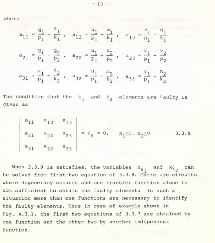
lll
21
31
given as
_ q i s _ U 1 m
V 1 n l Pi !<! 12
Pl ' a i3 = ^ - - li . 12 _ U 1 U 2 a - li - V 2
Pp P 2 / cX22
P 1 P 2 ' 23 Pl
P2
q4 1 2 _ U 1 m2 ^2
Pl k 2 / ^
32 Pl k 2
a - - ' 33 Pl k 2
ition that the
k l and
k 2 elements are faulty is
11 a 12 a13 21 a 22 a 23 =
aa - 0, x l— 0 ' x 2— 0 3.3.9 31 a 32 a 33
When 3.3.9 is satisfies, the variables x, and can
k l k 2
be solved from first two equation of 3.3.8. There are circuits where degeneracy occures and one transfer function alone is not sufficient to obtain the faulty elements In such a situation more than one functions are necessary to identify the faulty elements. Thus in case of example shown in
Fig. 4.3.1, the first two equations of 3.3.7 are obtained by one function and the other two by another independent
function.
Example of two faulty elements:
Consider the same example discussed in F i g . 4.3.1. Two elements are assumed fault. At a frequency m = l , the trans
fer function frequency response and input admittance fre
quency response is given as T (I ) 13
37 Y(I) _7
37 3 ■3! > lo' 6 y 3.3.10
14
we are required to identify the faulty component. This is a degenerate network where different combinations of R^, R2 and C may yield the same transfer function. Hence two different functions are used for identification. Three different possible sets are:
1 + Sx^
I+Sx^+3Sx2
R^ and R2
3.3.11 I + SC
0 are faulty
I+SC_R
0 R 10X 1 + SC^R (1+S) 1+Sx-^+3SX2
20C0 X 2X 3 l+Sx^
I+Sx3+3Sx2x3
R2 and C are faulty
3.3.12
1+SX 3 I+Sx3+3Sx2x3
15
resistor R^ and R2 are the faulty components. Their true value is R 1=2000 K, R 2=4000 K.
Case 2 . when R2 and C are considered faulty.
From T2 3(s) , A = B = 0, C = j / D = I » E = 3 j , H = I
p - M
- Q II O a 11 37 4 ' V = 2437k - If - L
11 0 s 11 2437 , N = - ■
The equations in variables x2 and are 12X3X3 + 4x^ = 24
39x2x3 -24X3 = 4 The solution is
X3 = 2 , x2 = 2 /3 From Y2 3(s) , which is same as T ^ i s )
P 15
37 , Q = 0 , U = 5/37 , v “ " 3730 21 , L = 0 , M = 30
, N 5
K 37 37 37
The two equations for variables x2 and
X 3 are 15x2x3 + 5X3 = 30
21x2X3 -30X3 = 5
yielding the solution X3=l , x2=5/3 . Since this solution is not the same as obtained from T ^ i s ) , the elements R2 end C are not the faulty elements as a pair.
16
Case 3 . and C are considers faulty.
From T31(s) , A = j to, B = 0, c = 0, D = 1 , E = jto, F = 0, G = j3o, H = 1 P = 3I , Q = 0 , u 12
37 , V = - 24 37 ' v _ _ 24 t _ _ M _ 39 M _ 4
^ 37 ' ^ 0 / M -y .
The equations in and x^, from the function T 3^(s) x. x_ + 3x^ = 6
1 3
- 24Xi x3 + 39x3 = 4 Thus
X x = 3/2 / x 3 = 4/3
From Y3i(s) • A = B = 0, U II -n 3 Q 11 rH W II -i—> 3 F = 0, G = j 3to, H = 1
P = 3 7 ' q = 0 '
U = 15
° 37 ' v = - 3° , 37 ' K - 37 ' L - °' M = - —
37 ' N - - 37 The equations in x^ and x 3 from the function Y 3^(s)
Xlx 3 + 3x3 " 6 = 0 7x lx 3 -16x3 “ 5 = 0 yielding x^ = 3 , x 3 = 1 .
The solution from Y 1 3 (s ) and T 1 3 (s ) do not agree with other, concluding that and C are not the faulty pair.
The conclusion reach is that R^ and R2 are the faulty resistors having actual value of 2000 K and 4000 K .
17
T31(s) = I+SR10C 0 X 1X 3
I+SR10C0X1X 3 + SR20C0 X 3
1+Sx3 l + S x 1x 3+ 3 S x 3
1 + SC x
Y (g) = --- y _^_________
3 1 v ' I+SR.^C^x., x _ + SR„_C_x, 10 0 1 3 20 O 3
R^ and C are faulty
1+Sx ^ l+Sx^x^+3Sx^
3.3.13
Case 1. R X and R2 are considered faulty
From t12(s)' A II w II u !i o D = H = I, B = F = j ' P = K = 0, Q = 4
37 7 a ii (jj|m
V = 24 37 .24 m _ 39
37 ' 37 , N 4 i_J
37
The equations for variables x-^ and x 2 , from the T ^ 2 (s), are
x^ + 3x2 = 6 -24x^ + 39x2 = 4 The solution is given as x^=2, x 2=4/3.
From Y 2 (s) P = 0, Q = 5/37, U = 15/37, V = -30/37 K = 0, L = 7/37, M = 21/37, N = -212/37 The two equations in variable x-^ and x 2 obtained from Y 1 2 (s ) degenerate into one equation
Xi + 3x2 = 6, which is satisfied by the solution x.^ = 2 and x 2 = 4/3, confirming that indeed the resistor R^ and R2 are the faulty components. Their true
18
3.4 Fault with three or more simultaneously faulty elements
With three faulty elements to be simultaneously identified either we need four different function to measured at one frequency (real and imaginary part) or one function at four different frequencies (if no degeneracy o c c u r e s ). In general for a m element fault 2m ^ measurements (real and imaginary part) of different functions, or one function test at 2
different frequencies is performed. For three element fault the equations obtained are of the form
a , ^ , x, x, x, + ai'V x, x, + aj V x, x, + k lk 2k 3 kl k2 k 3 k lk 2 k l k 2 k 2k 3 k 2 k 3
+ af1? x. x, + a f i ^x + a, x + k3k l k 3 k l k l k l k 2 k 2 . _ U ) X . _(i)_ n
+ ak 3 xk 3 + ao - °' 3.4.1
(l 1, . • • , 8) ,
( # k 3 , 'k 3 /k^ = 1,•..,n )
The product terms are eliminated by successive subtractions to obtain equations of the form
allXk 1 +
*12*k2 + a , x + a„ „X, +
21 k l 22 k 2 a , x + a „ „x. +
31 k x 32 k 2 a ., x,
41 + a..x 42 k 2 + The conditions that ]kl> k 2 and is given by
A, = det of A = 0, A = {a
a13Xk 3 a 14 = o a 24 = 0
3.4.2 a 34 = 0
a4 3 \ 3 + a 44 = 0
k 3 are the faulty elements
Ü 1' ( i 'ji=i,. . . ,4) 3.4.3
19
x > O, x > 0, x, > 0 3.4.4
K 1 K 2 K 3
The quanties x , x , x are solved from first three k 2 k 3
equations. The extension to m element fault is obvious.
4. CONCLUSION
A method has been presented for isolation of a fault when m elements are simultaneously faulty. In general 2 different measurements real and imaginary part are made to identify the faulty elements. In case the transfer function alone can not identify the faulty components, other functions such as input impedance or transfer function between different sets of terminals is used. Method is suitable for automatic fault identification via digital computer.
3 ° \ S j
20
REFERENCES
L ID Martens, G.O. and Dyck,J.D.S. "Fault Identification in Electronic Circuits with the Aid of Bilinear Transfor
mations", IEEE Trans, on Reliability, Vol. R-21, N o . 2, May 1972.
L 2d Sriyanands, H. , Towel1, D.R. and Williams, H.H. "Voting Techniques for Fault Diagnosis from Frequency-Domain Test-Data", IEEE Trans, on Reliability, Vol. R-24, No.4.
Oct.1975.
l3d Williams, H.H. "Transform Method of Computerized Fault Location", Conf. on "The Use of Digital Computers in
Measurement" University of York England, 24-27 Sept. 1973, IEEE London Conf. Publication No. 103.
c4d Lin, P.M. "A Survey of Applications of Symbolic Network Functions", IEEE Trans. Circuit Theory, Vol. CT-20, No. 6. pp. 732-737, N o w . 1973.
l5d Puri, N.N. "Rational Fault Analysis for Circuits and
Systems", to appear in April issue of Circuits and Systems Journal IEEE, 1976.
C63 Puri, N.N. "Fault Isolation in Electronic Equipment", Eighth Asilomar Conference on Circuits, Systems and Computers, pp. 584-588, Dec. 1974.
C 7 d Parker, S.R., Peskin, E., and Chirlian, P.M. "Application of Bilinear Transformation to network sensitivity", IEEE Trans. Circuit Theory /corresp./ Vol.CT-12, p p . 448-450, Sept. 1965.
L 8D Seshu, S. and Waxman, R. "Fault Isolation in Conventional Linear Systems - A feasibility study", IEEE Trans.Rel., Vol.R-15, p p . 11-16, May 1956.
19 D Gefferth, L. "Fault Identification in Resistive and Reactive Networks", Circuit Theory and Applications, Vol.2, pp. 272-277, 1974.