1
Geographical networks of international migration
Abstract
In the globalised world, various human activities (business, migration, etc.) organise into networks, and only through these skeletons can we observe the different phenomena that take place. In response to the emergence of globalisation we need to find new, usable tools and methods for the sound measurement of such changing phenomena. Network theory is an innovative approach that can help us handle the complexity of the 21st century. However, so far it has not featured in mainstream official statistics.
The international migration offers a new field, in which to harvest the results of network theory (in geographical not in sociological sense). Through the migration countries’ networks (from where and to where migrants move) I provide some of the most important tangible outcomes of network analysis in international migration statistics. The analysis of the entire migration geographical network is limited to the presentation of the main trends and characteristics.
Keywords: international migration, network theory, spatial networks, spatial statistics
1. Introduction
Migration is an interdisciplinary phenomenon, related mainly to demography, economics, history, geography, political science and sociology. Consequently, its interpretation and definition also emphasise different aspects. This article focuses more on geographical, statistical, mathematical-networking theoretical elements.
A detailed analysis of the root causes, main trends and potential effects of international migration is not the purpose of this study, it goes beyond its limits
The analysis of international migrants is often limited to foreign nationals living in a given country. Therefore, this study focuses on the foreign-born population (whether it is still of foreign national or citizen of the given country). The aim of the study is to present a network of migration relations between countries around the world and to examine the characteristics of this network. The analysis connects the sending and receiving regions and considers the phenomenon as a network, moreover it also tries to present its topology on a global scale by using 1990 and 2017 data.
2
The data underlying the analyses were obtained from the UN Migration Database (United Nations, 2017). The territorial unit of the analysis is the country. In this study, the UCINET NetDraw software was used to calculate and display networks (Borgatti et al., 2002).
2. The volume of international migration and connections among countries
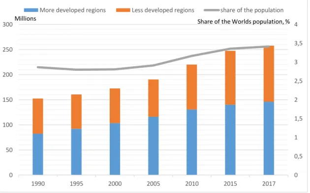
In 2017, 258 million people in the world did not live in the country in which they had been born. Most of them lived in developed countries. In 1990, 2.9% of the world’s population were international migrants, which increased to 3.4% in 2017. If trends of the 1990s and 2017s continue, by 2040, 372 million people will be international migrants, 4% of the world’s then- population.
Figure 1: Foreign born population in the World, 1990-2017
Source: UN, 2017
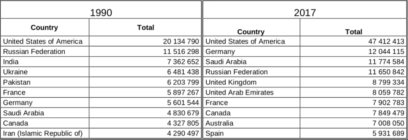
In 2017, the most foreign-born citizen lived in the USA, although Germany, Saudi Arabia and Russia also had a population of more than 10 million people of foreign origin. While in the USA, Germany, Canada and Saudi Arabia the number of foreign-linked populations doubled since 1990, in Russia, India, Iran, Ukraine, Pakistan their numbers stagnated or decreased.
0 0,5 1 1,5 2 2,5 3 3,5 4
0 50 100 150 200 250 300
1990 1995 2000 2005 2010 2015 2017
More developed regions Less developed regions share of the population
Millions Share of the Worlds population, %
3
Table 1: Top 10 receiving countries (persons), 1990, 2017
1990 2017
Country Total
Country Total
United States of America 20 134 790 United States of America 47 412 413 Russian Federation 11 516 298 Germany 12 044 115
India 7 362 652 Saudi Arabia 11 774 584
Ukraine 6 481 438 Russian Federation 11 650 842
Pakistan 6 203 799 United Kingdom 8 799 334
France 5 897 267 United Arab Emirates 8 059 782
Germany 5 601 544 France 7 902 783
Saudi Arabia 4 830 679 Canada 7 849 479
Canada 4 327 805 Australia 7 008 050
Iran (Islamic Republic of) 4 290 497 Spain 5 931 689
Most people move from countries with large populations, like India, China, Mexico, Russia, or from near crisis- and war zones. Migration in the 21st century is characterised by the increase in pensioner migration (Huber, O'Reilly, 2004; Illés, 2013) and that at older age from developed countries (e.g. the United Kingdom). Its main driving forces are the better use of the purchasing power of pensions, the recreational opportunities, or the search for a more favourable climate (Warnes, 2009).
Table 2: Top 10 sending countries (persons), 1990, 2017
1990 2017
Country Total Country Total
Russian Federation 12 664 537 India 16 587 720
Afghanistan 6 724 681 Mexico 12 964 882
India 6 718 862 Russian Federation 10 635 994
Ukraine 5 549 477 China 9 962 058
Bangladesh 5 451 546 Bangladesh 7 499 919 Mexico 4 394 684 Syrian Arab Republic 6 864 445
China 4 229 860 Pakistan 5 978 635
United Kingdom 3 795 662 Ukraine 5 941 653
Italy 3 416 421 Philippines 5 680 682
Pakistan 3 341 574 United Kingdom 4 921 309
Migration shows strong territorial concentration. In 2017 (like in 1990), 80% of migrants lived in 14% of the countries, while half of the migrant population lived in nine countries. In international migration there are centres (large receiver countries), global migration destinations that attract migrants from a greater distance. The foreign-born population living in these centres is diversified by country of birth. However, the relationship between volumes and migration relations among counties is more complexi.
Chile, as a destination country shows the largest interconnectedness in the world. In 2017, people from 210 different countries chose this country as their new residence. In Chile, almost
4
everyone except the Mapuche Indians is an immigrant or the descendant of immigrants. 16th- century Spanish settlers and those 19th-century Germans, followed by tens of thousands of Croats after the Dalmatian phylloxera epidemic emigrated to Chile. In the 20th century, many Europeans fleeing world wars and after them chose this country as their new home. These migration networks have survived to this day. Meanwhile, Chile has become the richest country in South America, thus, as a result of development, from the closer and more distant neighbours more and more people choose Chile as their new place of residence (Soltész, 2018, Aldunate et al., 2019)ii.
Table 3: Top 10 source - and sending countries with the most connections, 1990, 2017
1990
Destination Source
Country Number of connections
(source countries) Country
Number of connections (number of countries where a resident born in the source country
lives)
Australia 211 United States of America 157
Greece 209 United Kingdom 140
France 206 China 138
United Kingdom 203 France 135
Denmark 196 Canada 123
Chile 196 Germany 122
Canada 194 India 122
Austria 192 Italy 106
Italy 184 Australia 105
Ireland 179 Russian Federation 100
2017
Destination Source
Country Number of connections
(source countries) Country
Number of connections (number of countries where a resident born in the source country
lives)
Chile 210 United States of America 162
Australia 206 United Kingdom 146
United Kingdom 205 China 143
France 205 France 138
Canada 197 India 130
Ireland 195 Canada 127
Italy 193 Germany 125
Austria 192 Italy 111
Denmark 186 Australia 108
Greece 186 Russian Federation 102
The USA is acknowledged as a host country. Migrants from 150 different countries arrived in this centre territory, but people live in even more countries – 162 in total –who were born in the
5
USA. Large receiving countries, where the composition of immigrants by country of birth is diverse and have many inward links. People from Germany, the USA, Canada, France and Britain move to many other countries. This phenomenon can partly be explained by the migration at an older age as mentioned above and partly by the return of descendants of immigrants (Gmelch, 1980). However, this data also highlights that in the age of globalisation, migration is not a one-way movement.
Besides Chile, most countries of the European Union, as well as Australia are destinations, where people arrive from many different countries, however from there people migrate to few other countries still. People emigrate from countries with large population (China, India) and countries close to crisis zones (Syria, Ukraine, Somalia, Afghanistan) to many other countries (Sirkeci et al., 2015), while immigration takes place from relatively few countries (e.g. people living in India were born in 36 different countries, but those who were born in India live in 130 countries).
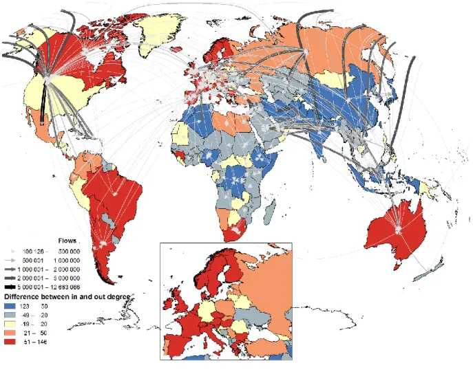
Connecting the source and destination areas is necessary to understand the characteristics of international migration. In this term, this conservative structure of the countries between two points of time (table 3) can help find out the internal features of international migration. There are also significant concentrations in the migration matrices presenting from and to trends between countries. The central role of the USA is demonstrated by the fact that as early as 1990, millions of people lived there who were born in Mexico (Massey, 2015) and Puerto Rico. From its population in 2017, the number of people born in China, the Dominican Republic, South Korea, India, Cuba, the Philippines, El Salvador, Puerto Rico, Mexico and Vietnam exceeded one million people per country. Germany also has more than one million people born in Poland, Kazakhstan, Russia and Turkey (Sirkeci et al., 2012) each. India’s role is twofold, to the USA, Oman, Kuwait, Saudi Arabia and the United Arab Emirates it is a major sending country, on the other hand millions arrive here from Bangladesh and Pakistan. Significant flows can be detected from Romania to Italy, from Myanmar to Thailand, from Palestine to Jordan, from Algeria to France, from Burkina Faso to Côte d'Ivoire, from Afghanistan to Iran and Pakistan, from Syria to Lebanon and Turkey. Movements usually take place towards wealthier areas.
Some of these links can be traced back to colonial times (Adeyanju, Oriola, 2011), in other cases leaving war zones plays an important role (Conte, Migali S, 2019). On average, the latter migrations are smaller, while the former involve longer distances.
6
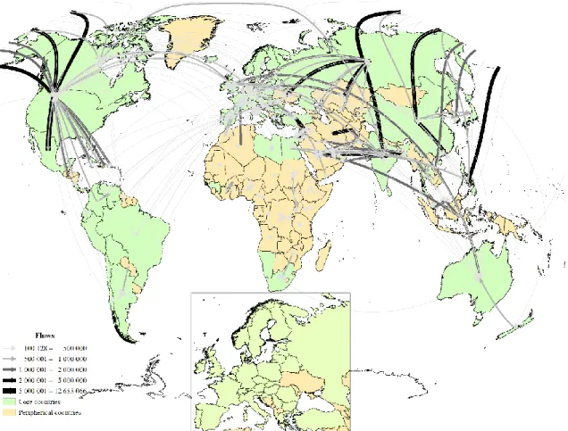
Figure 2: The relation between source and destination countries by the number of migrants, 2017
3. Geographical international migration networks
In the previous section, the foreign-linked population was examined according to the relationships of the country of birth and the current place of residence. In this chapter, the intrinsic characteristics of migration networks between countries are analysed in detail.
The analysis of the networks began in the second half of the 20th century (Erdős, Rényi, 1959, 1960; Bollobás, Erdős, 1976). It was an interesting and paradigm-shifting thesis of this era (Buchanan, 2003), that any two people on earth are connected by six steps away, called a familiarity relationship (six degrees of separation). After the initial graph theory, recent network theory at maths has become a new discipline with recognized abstractions. This was based on research showing that all networks, whether living or lifeless, in kind or artificial, are based on partially identical organizing principles. That is, the internet, human connections, the neuron network of the brain in their internal properties are very similar. (Barabási, 2008, 2016).
7
The network is the complexity of nodes and links that connect them in pairs. The degree of nodes represent the number of links a given node has to other nodes. The degree distribution (pk) plays a key role in network theory. The reason is that pk determines many network phenomena, from network robustness to the ability to evolve. The average degrees of a network can be expressed as:
〈𝑘〉 = ∑𝑁𝑖=1𝑖 ∗ 𝑝𝑖, where ∑𝑁𝑖=1𝑝𝑖 = 1 és 𝑝𝑖 =𝑁𝑖
𝑁 (Ni is the number of degree-i nodesiii)iv. In other form: 〈𝑘〉 =2𝐿
𝑁 , where L is the number of total links, N is the number of total nodes, because
𝐿 =1
2∑𝑁𝑖=1𝑘𝑖 , where ki is the degree of node-i.
Based on degree distributions, it can be theoretically differentiated between two types of networks: random and scale-free networks (Barabási, 2010). The degrees of a random network follow the Poisson distributionv:
𝑝𝑘 = 𝑒−〈𝑘〉∗〈𝑘〉𝑘
𝑘! ,
which in case of rare networks is similar to a bell curve. In other words, most nodes have about the same number of links and the probability of nodes with a large and small number of links is low. A national road system usually resembles a random network, where nodes are the settlements and links are highways (Barabási, 2008).
As with most networks, people-to-people links are most accurately described by the scale-free (power-law distribution) network:
𝑝𝑘 = 𝑘−𝛾
𝜁(𝛾), where 𝜁(𝛾) is the Riemann-zeta function: 𝜁(𝛾) = ∑∞𝑘=1𝑘−𝛾(Bombieri, 1992)vi. The degree distribution according to the power-law function predicts that most nodes in the network have only a few links to other nodes, which are held together by a few highly connected centres (Barabási, 2008). This peculiarity generates the ”small world” phenomenon. In other words, distance in a scale-free network is shorter than in a similar but randomly arranged one, so all nodes are close to the centres. Once these centres, the ”hubs” are present in a network, its behaviour will fundamentally be changed (Barabási, 2016, Battiston et al., 2017).
The key difference between random and scale-free networks is rooted in the different shapes of the Poisson and that of the power-law function. Random networks have an internal ”scale”. In
8
other words, nodes in a random network have comparable degrees, and the average degree 〈k
〉 serves as the ”scale” of the random network. Scale-free networks lack a scale; thus, the average degree does not advise us so much on the network. When a node is randomly selected, we do not know what to expect: the selected node’s degree could be tiny or arbitrarily large.
Hence, networks do not have a meaningful internal scale, but are “scale-free” (Barabási, 2017).
The presence of hubs and the small world phenomenon are universal characteristics of the scale- free network.
For the study, network theory is paramount because of the links between countries connected by international migration. Thus, nodes are the countries. There is a link between two countries if international migration between these two countries exist, i.e. someone moved from his/her place of birth to the other country, his/her current place of residence with certain restrictions, regardless of how many people moved. The unweighted network considers movements above a threshold. The reason is that a small number of international migrants do not necessarily mean a real migration relationship between two big countries. Namely, two countries are only connected in the net by edge, if the number of migrants between the two countries is relevant and asymmetric, ie
𝑞(𝐴, 𝐵) =𝑀[𝐴 → 𝐵] − 𝑀[𝐵 → 𝐴]
𝑁(𝐴) + 𝑁(𝐵)
is above a µ fixed threshold. Where 𝑀[𝑋 → 𝑌] is the number of population born in country X and living in country Y, N(X) is the resident population of country, 𝜇 ∈ {−1; +1}, 𝜇 ∈ 𝑹.
If q (A, B)> μ, a migration bond is created from country A to country B, and if not, there is no such link between the two countries. This allows different nets to be edited depending on the μ parameter.
An analysis of the country’s relations systems presents how diverse migration is, how
”embedded” the process is in the region. Links between countries and those dynamics involve changes in the volume of future migrations. In case of degree reduction (if a country will have fewer links to other countries due to migration) it is likely that the respective sending areas are depleted or the receiving countries are saturated, the earlier migration waves were reduced or other areas became more attractive to new arrivals. Provided that degrees increase, the number of links increases, which may foresee further increase in the number of migrants due to the growth of the potentially accessible population.
9
By determining the degrees, it is possible to examine how many countries have a given number of degrees (links). The question is whether it is possible to find a random, scale-free or other kind of topology.
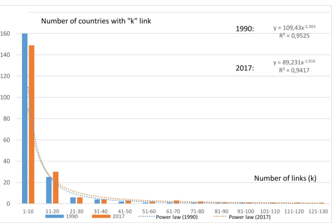
Figure 3: Degree distribution of immigration by country, 1990, 2017
The number of countries with a given number of links decreases by the number of links by quasi-power law functionvii, the network of (im)migrations is scale-free with a good approximationviii. In such scale-free networks, the average degree does not provide sufficient information about the network. For a randomly chosen country, the number of expatriate population living there may be very low or high. This means that there is no country of average migration.
The reason for scale-free topology found in the migration network is that countries with multiple links will be much more attractive to migrants than those with fewer degrees.
Integration into the new environment is successfully achieved where it is facilitated by previous family and friendly relationships. The ”beaten track” of emigration is to liaise with those already displaced, which also has a significant impact on future migration decisions (Haug, 20018; Rédei, 2007; Kiss, 2007). This is justified by the fact that family reunification is still one of the main purpose of accessing a country, while on the other hand, the new arrivals often
y = 109,43x-2,303 R² = 0,9525
y = 89,231x-1,916 R² = 0,9417
0 20 40 60 80 100 120 140 160 180
1-10 11-20 21-30 31-40 41-50 51-60 61-70 71-80 81-90 91-100 101-110 111-120 121-130
1990 2017 Hatvány (1990) Hatvány (2017)
1990:
2017:
Number of countries with "k" link
Number of links (k)
Power law (1990) Power law (2017)
10
settle near their relatives and acquaintances. So with more links to a country, migration is much more effortless, a larger number of potential migrant population and information can be accessed through family, friends, relatives and acquaintances. A migrant is more likely to choose a popular country or settlement with many connections, about which more information is available than one that he or she knows little about. Thus, the emergence of migration networks can be the main influence on the direction and volume of migrations, in addition to income disparities and migration distances.
4. Topology of migration networks
Once the scale-free peculiarity was recognized in the degree distribution of migration networks, it is possible to examine in detail the intrinsic characteristics, the topology of the networks (density, centralisation, distance between nodes, centre-periphery test, centralisation), moreover it is also possible to draw conclusions on some the nature of international migration.
The density of a networkix is the total number of existing ties divided by the total number of possible ties (each country would be linked to all other countries by migration).
Table 4: Density of the migration network, 1990, 2017
Year Density Deviation (SD)
1990 0.033 0.789
2017 0.045 0.2072
In 2017, the density of the migration network was 4.5%. Connectivity is constantly increasing, migration help expand relationships between countries and people’s flow between countries is intensified. There is also migration between areas where there was no link in the past.
The applied programme used can help us calculate how far each country is on average through migrationx (the geodesic distance between two countries is the length of the shortest migration route between them and the route between two points equals the number of contacts). For example, the distance between the USA and China is one because there is one person living in the USA who was born in China, however the distance of Albania and Afghanistan is two (there is no direct migration between the two countries), people migrate from Afghanistan to Italy and then from Italy to Albania. This peculiarity is asymmetrical for managed networks, the distance
11
between Afghanistan and Albania is three: people move from Albania to Georgia, from Georgia to Tajikistan and then from there to Afghanistan.
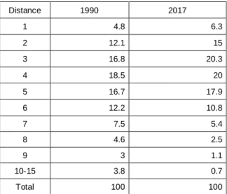
The average distance between countries was 4.667 in 1990 and reduced to 4.075 in 2017. This also means that the interconnectedness of the countries is significant and has increased slightly during the period considered. Countries around the world have an average of 4 migration links, with nearly 21% of all potential pairs of countries directly or through another country.
Table 5: Distance of migration between countries (%), 2001, 2017
Distance 1990 2017
1 4.8 6.3
2 12.1 15
3 16.8 20.3
4 18.5 20
5 16.7 17.9
6 12.2 10.8
7 7.5 5.4
8 4.6 2.5
9 3 1.1
10-15 3.8 0.7
Total 100 100
With help of density within the migration network we can determined the considering centre and peripheral areas. This is based on an iterative procedure that divides the countries of the network into two parts in such a way that the density of the centre part is maximumxi.
Table 6: Density rates of centre-peripheral areas, 2017
2017 centrum periphery
centrum 0.326 0.019
periphery 0.102 0.022
According to the procedure, North America, the greater part of Europe, Australia, New Zealand, Israel, South Africa, Russia, Turkey, Philippines, Syria, Iraq, Lebanon and Sri Lanka belong to the core areas, while in this respect the other countries can be considered peripheral area. The links between the centre areas are strong, while there is almost no link between the other areas.
On the other hand, there is a considerable migration from the peripheral area to the centre, the density of this is five times the rate of reverse movements.
12
Figure 4: Centre and peripheral areas in international migration, 2017
While density expresses a general level of network cohesion, centralisation the extent to which connections are clustered around nodes. Centralization - or rationalization of the network - demonstrates how unequal is the distribution of the connections of the items (on a scale of 0- 100, where 100 represents a fully centralized network). The analysis was also carried out on a directional and symmetrical network. The designation of out degree refers to emigrations, while network indegree to the analysis by immigrations, and in symmetrical cases the relationship between two countries is independent of the direction of migration.
Table 7: Centralization in migration networks (%), 1990, 2017
1990 2017
Out degree 11,9 10,7 In degree 36,69 52,01 Symmetric 34,39 48,57
Emigrations are much less concentrated than immigration. The moderately strong degree of centralisation shows that most countries have few links with other countries through migration (numerous small degree nodes), while few have many links. The network is, however not fully
13
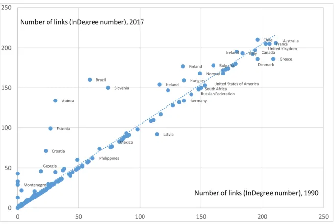
centralised and none of its members has an unlimited growing relationship collecting potential or monopoly. Furthermore there are several central elements of the network, and there is room for ”link-enhancing competition” between the elements. After all, the connection within the network varies, some countries are more connected to others, while others may lose their attractive abilities. Examples of the former one are Guinea, Estonia, Brazil and Slovenia, while Latvia, Denmark or Greece are countries that have lost some of their attractiveness. This, nevertheless does not mean that it is also associated with a reduction in the number of migrants every time, as more people can arrive through fewer connections.
Figure 5: Number of migration source countries of a given country, 1990, 2017
5. Conclusions and discussions
Migration shows strong territorial concentration, in 2017 half of the migrant population lived in nine countries. There are centres (large receiving countries) in international migration, global migration destinations that attract migrants from a greater distance.
Chile, most countries of the European Union, Australia, Brazil, South Africa are the countries where people arrive from many places, however from there people migrate just to few other
Australia
Greece France United Kingdom Chile
Denmark Canada Italy Ireland Bulgaria
United States of America Norway
South Africa Russian Federation Hungary
Germany Finland
Iceland
Latvia Mexico
Philippines Slovenia Brazil
Guinea
Estonia
Croatia Georgia
Montenegro
0 50 100 150 200 250
0 50 100 150 200 250
Number of links (InDegree number), 2017
Number of links (InDegree number), 1990
14
countries. People emigrate from countries with large populations and countries close to crisis zones to many other countries, while immigration takes place from relatively few countries.
Large receiving countries, where the composition of immigrants by country of birth is diverse and countries have many inward links, are often widespread sending ones themselves. This phenomenon can partly be explained by old-age migration and partly by the return migration of descendants whose ascendants emigrated here. This data however, also highlights that, in the age of globalisation, migration is not a one-way action.
The global international migration network has a scale-free topology. Countries with multiple links will be much more attractive to migrants than those with fewer degrees. The ” beaten track” of emigration is to liaise with those already displaced. A migrant is more likely to choose a popular country or settlement with many links, about which more information is available than one that he or she knows little about.
The interconnection between countries is constantly growing, migration is expanding relations between countries and people’s movement between countries is escalating. Migration also takes place between areas where there was no previous connection. As a result, the average migration distance between countries was reduced to 4 in 2017. More than one fifth of all possible country pairs are related directly or through another country.
The moderately strong degree of centralisation of the world’s migration network shows that most countries have few links with other countries through migration (numerous small degree nodes), while few have many links. The global network is, however not fully centralised and none of its members has an unlimited growing relationship collecting potential or monopoly.
There are several central elements of the network, and there is room for ”link-enhancing competition” between the elements. After all, the connection within the network varies, some countries are more connected to others, while others may lose their attractive abilities. This, nevertheless does not mean that this is also associated with a reduction in the number of migrants every time, as more people can arrive through fewer connections. The global scale- free type of network is much more resilient to external influences (due to multiple centres), so as long as migration has a driving force, international migration will strengthen in the current global regulatory environment, and its directions can slightly and locally be influenced.
In the globalised world, various services and phenomena (Internet, migration, business, electricity supply, mobile phone calls etc.) fall into networks with scale-free topology, centres and small world phenomena can be discovered. In these cases, it may be useful to bear in mind
15
the universal peculiarity of these networks and their consequences because complex systems and their collective behaviour cannot be fully recognized purely from the outputs of the components of the system.
It is therefore essential to recognise that in case of the power-law distribution, observation units are not of the same importance, and that more attention should be paid to global networks, nodes, key units to learn the phenomenon more precisely.
Acknowledgements: This study was supported by the Bolyai Research Fellowship of Hungarian Academy of Science.
References
1. Conte, A., Migali, S. (2019): “The role of conflict and organized violence in international forced migration”, Demographic Research Volume 41, Article 14: 393-424, DOI: 10.4054/DemRes.2019.41.14 Research Article
2. Barabási, A. L. (2008): Behálózva. Helikon Kiadó, Budapest, p. 320.
3. Barabási, A. L. (2010): Bursts: The Hidden Pattern Behind Everything We Do; Button, New York; p. 310 4. Barabási, A. L. (2016): Network Science, Cambridge University Press, p.453
5. Barabási, A. L. (2017): A hálózatok tudománya, Libri, Budapest, p. 444.
6. Battiston, F., Nicosia, V., Latora, V. (2017): “The new challenges of multiplex networks: Measures and models.” The European Physical Journal Special Topics. 226 (3): 401–416. doi:10.1140/epjst/e2016- 60274-8. ISSN 1951-6355.
7. Bollobás, B., Erdős, P. (1976): “Cliques in Random Graphs”. Math. Proc. Cambridge Phil. Soc. 80 (3):
419–427.
8. Bombieri E. (1992): “Problems of the Millennium: the Riemann Hypothesis”, Institute for Advanced Study, Princeton, NJ 08540:
https://www.claymath.org/sites/default/files/official_problem_description.pdf
9. Borgatti, S. P., Everett, M. G., Freeman, L. C. (2002): Ucinet 6 for Windows: Software for Social Network Analysis. Harvard, MA: Analytic Technologies.
10. Buchanan M. (2003): Nexus, avagy kicsi a világ. Typotex, Budapest, p. 236.
11. Adeyanju, C. T., Oriola, T. B. (2011): “Colonialism and Contemporary African Migration: A Phenomenological Approach”, Journal of Black Studies, Vol. 42, No. 6 (September 2011): 943-967.
12. Massey, D. S. (2015): “A Missing Element in Migration Theories”, Migration Letters, 12/2015, No 3:
279-299
13. Erdős, P., Rényi A. (1959): „On Random Graphs. I.”. Publicationes Mathematicae 6: 290–297.
14. Erdős, P., Rényi A. (1960): “On The Evolution of Random Graphs.” Magyar Tudományos Akadémia Mat. Kutató Int. Közl. 5: 17–61.
15. Gmelch, G. (1980): “Return Migration”, Annual Review of Anthropology, Vol. 9: 135-159
16
16. Haug, S. (2008): “Migration Networks and Migration Decision-Making”, Economics in Migration Research: Prospects for Disciplinary Integration, Volume 34, 2008 - Issue 4: 585-605
17. Huber, A., O'Reilly, K. (2004). “The construction of Heimat under conditions of individualised modernity: Swiss and British elderly migrants in Spain”, Ageing and Society, 24(3), 327-351.
doi:10.1017/S0144686X03001478
18. Illés, S. (2013): Időskori nemzetközi migráció – magyar eset. Tullius Kiadó, Budapest, p. 240 19. Kiss, T. (2007): “Demográfiai modellek és a migráció”. Régió, Vol 18. No 2.:160–189.
20. Rédei, M. (2007): Mozgásban a világ, a nemzetközi migráció földrajza. Eötvös Kiadó, Budapest, p. 568.
21. Aldunate, R., Contreras, G., De la Huerta, C., Tapia, M. (2019): “Characterization of the Recent Immigration to Chile.” No 830 Enero 2019 BANCO CENTRAL DE CHILE, Working Papers of the Central Bank of Chile Agustinas 1180, Santiago, Chile p. 26
http://si2.bcentral.cl/public/pdf/documentos-trabajo/pdf/dtbc830.pdf
22. Sirkeci, I., Cohen, J.H., Yazgan, P. (2012): “Turkish culture of migration: Flows between Turkey and Germany, socio-economic development and conflict”, Migration Letters, 9/2012, No 1: 33-46
23. Sirkeci, I., Yazgan, P., Utku, D.E. (2015): “Syrian Crisis and Migration”, Migration Letters, 12/2015, No 3: 181-192
24. Soltész, B. (2018): “Chilei fejtörő Bevándorlás – másként”, Földgömb, 36. évfolyam, 3. szám, pp. 42-53.
http://epa.oszk.hu/03000/03037/00049/pdf/EPA03037_foldgomb_2018_03_040-053.pdf
25. United Nations, Department of Economic and Social Affairs. Population Division (2017): Trends in International Migrant Stock: The 2017 revision (United Nations database, POP/DB/MIG/Stock/Rev.2017).
26. Warnes, T. (2009): “International Retirement Migration.” In: Uhlenberg P. (eds) International Handbook of Population Aging. International Handbooks of Population, vol 1. Springer, Dordrecht, pp 341-363
i Between 1990 and 2017, the number of migrants increased by 71.6%. The number of migration links between countries increased by 7.9% and the average number of migrants across one migration connection increased by 58.9%.
ii In Chile mass protests began in October 2019 due to the increase in the price of metro tickets. Demonstrations are driven by large inequalities in the country, low pensions and salaries, as well as high prices for electricity, gas supply, university education and health care.
iii 𝑁𝑖= 𝑁 ∗ 𝑝𝑖
iv Once the average degree exceeds ‹k› = 1, a giant component should emerge that contains a finite fraction of all nodes. Hence only for ‹k› › 1, the nodes organize themselves into a recognizable network. For ‹k› › lnN all components are absorbed by the giant component, resulting in a single connected network.
v if 〈𝑘〉 ≪ 𝑁 the distribution is binomial.
vi Details on zeta function are available at: http://mathworld.wolfram.com/RiemannZetaFunction.html
vii Calculated with µ=0,006 which means that in the migration network those links were taken into account, where the difference of migrant population between the two given countries exceeds 0,6% of the resident population of these countries.
viii In 2017: µ=0,004, R2=0,896; µ=0,005, R2=0,913; µ=0,006, R2=0,942; µ=0,007, R2=0,937. Thus hereafter µ=0,006 was applied as threshold.
ix The density of a binary network is the total number of ties divided by the total number of possible ties. For a valued network it is the total of all values divided by the number of possible ties. The density of a network is simply the average value of the binary entries and so density and average value are the same. If the network or matrix has been partitioned this routine finds these values within and between the partitions. This is the same as finding the average value in each matrix block. The routi ne will perform the analysis for non-square matrices (Borgatti et al., 2002).
x The length of a path is the number of edges it contains. The distance between two nodes is the length of the shortest path. The distance matrix can be converted to a nearness matrix by taking reciprocals of the distances.
xi Fits a core/periphery model to the data network, and identifies which actors belong in the core and which belong in the periphery. The algorithm uses in-degree for binary data as a starting partition and eigenvector for valued data together with a number of random partitions. A hill climbing technique is used to improve the initial partitions and the best fit is reported. The fit function is the correlation between the permuted data matrix and an ideal structure matrix consisting of ones in the core block interactions and zeros in the peripheral block interactions (Borgatti et al., 2002).