Ecological Informatics 44: 1-6. (2018) 1
2
Through the jungle of methods quantifying multiple-site resemblance 3
4 5
Dénes Schmera1,2 & János Podani3,4 6
7 8
1MTA Centre for Ecological Research, Balaton Limnological Institute, Klebelsberg K. u. 3, H- 9
Tihany, Hungary, E-mail: schmera.denes@okologia.mta.hu 10
2MTA Centre for Ecological Research, GINOP Sustainable Ecosystem Group, Klebelsberg K. u.
11
3, H-Tihany, Hungary 12
3Department of Plant Systematics, Ecology and Theoretical Biology, Institute of Biology, L.
13
Eötvös University, Budapest, Hungary 14
4MTA-ELTE-MTM Ecology Research Group, Budapest, Hungary 15
16 17
Abstract 18
Methods that quantify multiple-site resemblance are basic toolkits of ecology for studying 19
community variation in space and time. Although both pairwise and multiple-site 20
coefficients have received increasing attention in the past decade, the high variety of 21
methodologies combined with the absence of a systematic review prevents full 22
understanding and comprehension. To illuminate the situation, we compare and classify 23
methods that use incidence data and propose a unified terminology. The methods can be 24
grouped according to families, approaches and forms. The examination of algebraic 25
expressions and analyses of artificial and actual data sets suggest that inference drawn 26
about communities strongly depends on the methodology applied. We found that the 27
impact of mimicking the original pairwise indices (i.e. the impact of families) was stronger 28
than the impact of components used in formulating the coefficients (i.e. the impact of 29
approach). Our findings suggest that the measures examined quantify drastically different 30
facets of multiple-site resemblance and therefore they have to be selected with care in 31
community studies.
32 33
Keywords 34
community resemblance, community variation, dissimilarity, multiple-site resemblance 35
coefficients, pairwise resemblance coefficients, similarity 36
37 38
1. Introduction 39
40
Understanding spatial variation in species composition is one of the most fundamental 41
challenges of community ecology. This is promoted by testing hypotheses about the 42
processes that generate and maintain biodiversity in ecosystems (Legendre & De Cáceres, 43
2013). Invasion ecologists, for instance, examine the impact of alien species on native 44
communities, while conservation biologists rely on the measurement of compositional 45
variation in prioritizing areas. The spatial variation of communities can be viewed as either 46
compositional differentiation or similarity (Jost et al., 2011). Beta diversity (Whittaker, 1960, 47
1972), for instance, expresses compositional differentiation, while community overlap (Arita, 48
2017, Schmera, 2017) relates to compositional similarity – which are two sides of the same 49
coin.
50 51
Community variation has been traditionally studied by examining several pairs of sites from 52
the same locality (but see Legendre & De Cáceres, 2013, for alternative solutions) and 53
quantified by the average value of pairwise resemblance (i.e., similarity or dissimilarity) 54
coefficients (Koleff et al., 2003). Such averages may be used to express both compositional 55
similarity and differentiation. Recently, however, it has been suggested that inference drawn 56
from mean values may be misleading, because pairwise resemblance coefficients cannot 57
account properly for co-occurrence patterns of species in many sites and therefore special 58
indices are required (Diserud & Ødegaard, 2007; Baselga, 2013).
59 60
Although multiple-site resemblance coefficients have received increasing attention in 61
contemporary ecology, our knowledge on their relative merits and potential disadvantages is 62
still limited. A recent review on beta diversity deliberately omitted their discussion (Legendre 63
& De Cáceres, 2013) while an even more recent study deepened our understanding of 64
multiple-site overlap measures by providing novel measures and a unified terminology 65
(Arita, 2017). Unfortunately, however, the increasing number of methods, the application of 66
different and often overcomplicated mathematical equations, the ambiguous terminology, 67
as well as the parallel development of similarity and dissimilarity forms impede proper 68
measurement of multiple-site resemblance. Therefore, for the benefit of practicing 69
ecologists, we review the methods quantifying multiple-site resemblance that are based on 70
incidence (presence-absence) data. First, we discuss some basic terms, then we overview 71
pairwise and multiple-site resemblance coefficients. Specifically, we identify and match 72
similarity and dissimilarity forms and simplify some equations. Finally, by using artificial and 73
actual data sets we compare the performance of multiple-site resemblance measures.
74 75 76
2. Basic terms 77
78
Originally, pairwise and multiple-site resemblance coefficients have been suggested to 79
measure the (dis)similarity of two or multiple sites based on the presence-absence of 80
species. Consequently, sites are the objects of such studies and species are the descriptors 81
which characterize the objects. Observed data are commonly arranged in matrix X ≡ {xij}, in 82
which rows represent sites while columns correspond to species (e.g. Legendre & DeCáceres, 83
2013), a convention followed here as well. Occurrence (of species j in site i) means that 84
species j is present in site i, coded as xij = 1. In case of species absence, xij = 0. The species 85
richness of site i (ti) is the number of occurrences in the given row (row total,
T
1
j ij
i x
t ,
86
where T is the number of species). The occurrence frequency of species j (nj) is the number of 87
sites in which the species is present (called also as range size and calculated as the column 88
total,
N
i ij
j x
n
1
, where N is the number of sites). Whereas co-occurrence is traditionally 89
understood as the presence of a pair of species in a given site (Mackenzie et al. 2004, Bell 90
2005, Pollock et al. 2014 and references therein), Arita and co-workers (Trejo-Barocio & Arita 91
2013, Arita 2017) termed co-diversity, with a reference to Bell (2005), as the occurrence of a 92
species in two sites. It follows that the number of co-occurrences in a site is the number of 93
species pairs present there, while the number of co-diversities is the number of unique site- 94
pair occupancies of a given species. In a more formal way, the number of co-occurrences in 95
site i can be expressed as 96
2 ti
, Eq. 1
97
while the number of co-diversities of species j as:
98
2 nj
. Eq. 2.
99
Furthermore, following Schmera (2017) we consider community overlap as a phenomenon 100
that represents the intersection in the composition of sites, overlapping species as species 101
with at least two occurrences in a set of sites, overlap size as a quantitative property of 102
overlapping species that is quantified as the occurrence frequency of the given species 103
minus one:
104
1
nj , Eq. 3.
105
and total overlap size as a quantitative property of community overlap 106
T n
T j
j
1. Eq. 4.
107
108 109
3. Pairwise resemblance coefficients: a short overview 110
111
The literature of numerical ecology abounds in resemblance coefficients (sensu Orlóci 1972) 112
for comparing pairs of sites based on their species composition. We are concerned here with 113
similarity (s) and dissimilarity (d) forms which are bounded between 0 and 1, and are 114
therefore complements (d + s = 1). Presence-absence versions are commonly expressed in 115
terms of a 2 x 2 contingency table in which a refers to the number of species present in both 116
sites being compared (shared species, or the number of overlaps in species composition), b 117
to the number of species present only in the first and c to the number of species in the 118
second. That is, with respect to a given pair of sites there are b and c species unique to the 119
first and to the second site, respectively, so that the total number of species in the two sites 120
equals to a + b + c. We shall focus on three well-known resemblance coefficients, namely the 121
Jaccard, the Simpson and the Sørensen indices (Table 1, see Koleff et al. 2003 for further 122
indices).
123 124 125
4. A proposal for a unified terminology to classify methods quantifying multiple-site 126
resemblance 127
128
Here we suggest a unified terminology that allows the classification of methods quantifying 129
multiple-site resemblance. The multiple-site indices (see next paragraph for details) 130
mimicking some properties of the original pairwise Jaccard, Simpson and Sørensen indices 131
(Table 2) are termed as different groups (Legendre 2014), types (Arita 2017) or families 132
(Baselga, 2012, Baselga & Leprieur, 2015, Podani & Schmera, 2016). This confused 133
nomenclature, however, does not support the development of the field. We therefore 134
suggest, following the terminology of the first classifier (Baselga 2012), that classes of 135
methods mimicking some properties of the original pairwise coefficients should be termed 136
as families. Accordingly, the methods in question can be classified into Jaccard, Simpson and 137
the Sørensen families.
138 139
Families, however, do not provide the only way for classifying multiple-site resemblance 140
measures. The next feature on which further grouping is made depends on the type of 141
components (mathematical terms) incorporated into the coefficient. Some of the measures 142
rely only upon pairwise components, some use only general components of the studied 143
presence-absence matrix such as the total overlap size, others use co-diversity and, finally, 144
further ones combine general and pairwise components (see next paragraph for details). We 145
suggest that classes of methods formed according to the components used should be 146
termed as approaches, and we can distinguish among mean pairwise, general, co-diversity 147
and mixed components approaches (see below). Finally, as said above, each coefficient can 148
be expressed as similarity or dissimilarity. We will refer to this property of coefficients as 149
forms.
150 151
Consequently, we suggest a classification of methods quantifying multiple-site resemblance 152
according to families, approaches and forms. The terminology becomes even more complex 153
if we consider that dissimilarity forms (also used as measures of beta diversity) may be 154
partitioned into additive components to separate the effect of various background factors 155
influencing dissimilarity. There are two different frameworks for such a partitioning, 156
intensively discussed and debated in the relevant literature (Baselga, 2010, Carvalho et al., 157
2013, Cardoso et al., 2014, Ensing & Pither, 2015, Chen, 2016, Podani & Schmera, 2016).
158 159 160
5. Multiple-site resemblance: a new classification 161
162
Here we suggest a classification of methods assessing multiple-site resemblance by 163
considering families, approaches and forms. In this, we do not suggest any hierarchy among 164
these categories. The classification includes both pairwise and multiple-site coefficients.
165
Pairwise coefficients are used for quantifying multiple-site resemblance by calculating the 166
mean of pairwise coefficients, referred here as "mean pairwise approach".
167 168
Multiple-site coefficients express resemblance of more than two sites simultaneously (Table 169
2). Although the first multiple-site index dates back to the 1950's (Koch 1957, see also Eq.
170
Tab2/1), further elaboration of such coefficients has started only recently. Some of the new 171
indices follow the logic of pairwise indices and therefore we categorize them into the 172
Jaccard, Simpson and Sørensen families (Table 2). However, the coefficients in either family 173
use different components in quantifying similarity or dissimilarity. In studying the overlap of 174
multiple sites, for instance, Arita (2017) suggested general overlap indices, which use only 175
some general components of the incidence matrix, as well as co-diversity indices, which use 176
the occurrence of two species at a particular site. In other studies, Baselga and co-workers 177
(Baselga et al. 2007, Baselga 2010, 2012) used both general and pairwise components in 178
expressing multiple site resemblance or, in other words, they used mixed components. As 179
said above, we refer to this property of coefficients as approach and distinguish among 180
mean pairwise (Table 1), general, co-diversity and mixed components approaches (Table 2).
181
Note that we use the term general instead of general overlap (sensu Arita 2017), because 182
“general” can reflect both similarity and dissimilarity, whereas “general overlap” intuitively 183
relates to similarity only. Thus, we can distinguish three families (Jaccard, Simpson and 184
Sørensen), four approaches (mean pairwise, general, co-diversity and mixed components) 185
and two forms (similarity and dissimilarity) of methods quantifying multiple site resemblance 186
(Tables 1 & 2).
187 188
General similarity indices belonging to different families may be formalized in different ways 189
(Table 2). The observed total overlap size (Eq. 4) may be divided by the maximum number of 190
total overlap size with N sites and T species (Jaccard family, Eq. Tab2/1), or by the maximum 191
number of total overlap sizes possible if the sites show a nested design (Simpson family, Eq.
192
Tab2/3). Thirdly, average overlap size of species may be divided by the average species 193
richness of sites (Sørensen family, Eq. Tab2/4).
194 195
Baselga and co-workers (Baselga et al. 2007, Baselga 2010, 2012), following Diserud &
196
Ødegaard (2007), used
i
i T
t as the "number of shared species" in the multiple-site 197
situation. Since
N i
ti 1
=
T j
nj 1
= G, the grand total of X (see also Arita et al., 2008, 2012; Arita 198
2017), we can call
i
i T
t as total overlap size (Eq. 4). Multiple-site "unique species", 199
however, were quantified as the sum of unique species for pairs of sites. It follows that it is a 200
mixed components approach having both pairwise and general constituents. A possible 201
theoretical problem with this is that total overlap size (from the general approach) and the 202
number of site pairs in which the same species occur (pairwise component, called also as co- 203
diversity [Arita 2017]) in the data matrix are not the same (Arita 2017), and therefore the 204
ecological interpretation of these indices is less straightforward.
205 206
Moreover, in addition to general indices, Arita (2017) developed a new approach of multiple- 207
site similarity measures he called the co-diversity indices. These indices, in fact, count the 208
sum of the two-site occurrences (co-diversity) of species which is divided either by the sum 209
of the co-diversities when site compositions show a nested design (Simpson family, Eq.
210
Tab2/10), by the possible number of co-diversities when N sites are occupied with T species 211
(Jaccard family, Eq. Tab2/9) or, finally, by the sum of average species richness for each pair 212
of sites (Sørensen family, Eq. Tab2/11).
213 214 215
6. Simplification of some equations 216
217
A couple of mixed-component resemblance coefficients have originally been published with 218
extensive mathematical equations. To make their use easier, we suggest the simplification of 219
two functions. The mixed component Jaccard dissimilarity (Eq. Tab2/6) suggested by Baselga 220
(2012) can be simplified to 221
i k l
lk kl i
l k
lk kl
b b T
t
b b
) (
) (
) (
, Eq. 5.
222
while the mixed component Sørensen dissimilarity (Eq. Tab2/8) suggested by Baselga (2010) 223
reduces to 224
i k l
lk kl i
l k
lk kl
) b b ( ) T t ( 2
) b b (
Eq. 6.
225
226 227
7. Comparison of methods quantifying multiple-site similarity 228
229
7.1 Methods to compare 230
Here we compare methods that allow quantification multiple-site resemblance. Although we 231
use similarity forms, our conclusions are not restricted to similarity because it is 232
complementary to dissimilarity. Although pairwise coefficients are designed for examining 233
pairs of sites, the mean values of these coefficients are frequently used for assessing 234
multiple site similarity. We will refer to this as mean pairwise approach. We examined also 235
general, mixed components and co-diversity approaches, as well as the Jaccard, Simpson and 236
Sørensen families. In sum, we define any particular method as the combination of an 237
approach and a family, and thus compared 12 methods.
238 239
7.2 Artificial data 1 240
To compare the performance of methods, we examined all possible communities that can be 241
produced by the co-occurrence of 4 species in 4 sites. In order to calculate the number of 242
possibilities, we have to first determine how many ways a single species can be distributed in 243
N sites. Since there are two outcomes for each site (the species is present or absent), the 244
possible number of occurrence patterns equals 2N. However, this includes the situation 245
when the species is absent from all sites. Therefore, the number of occurrence patterns 246
reduces to 2N-1 (for N = 4 we have 15 different patterns). When we have T species, then the 247
possible number of co-occurrence patterns increases dramatically (2N-1)T (for N = T = 4 we 248
get 50,625). However, these co-occurrence patterns include empty sites (those without 249
species) as well. After removing degenerate matrices, the number of meaningful co- 250
occurrence patterns reduces to 41,503 in the example.
251
252
We calculated multiple-site similarities by the different methods (i.e. the combinations of 253
families and approaches) for each of the 41,503 occurrence patterns. When no similarity 254
form was given (the Jaccard and Sørensen families of mixed components), we used the 255
complement of dissimilarity. The resulting scores served as a data set to calculate the 256
Pearson correlation between different methods, in order to express agreement in trends 257
among the measures. We transformed the correlations to distances (distance = 1 – 258
correlation) and analyzed the distance matrix by UPGMA clustering to obtain a dendrogram.
259
The same distance matrix was analyzed by principal coordinates analysis (PCoA). Thus, in 260
these multivariate studies, each object represents a given measure. We used the gtools 261
(Warnes et al. 2014), the betapart (Baselga et al. 2013) packages in R (R Core Team, 2015) 262
and the SYN-TAX 2000 package (Podani 2001) for computations.
263 264
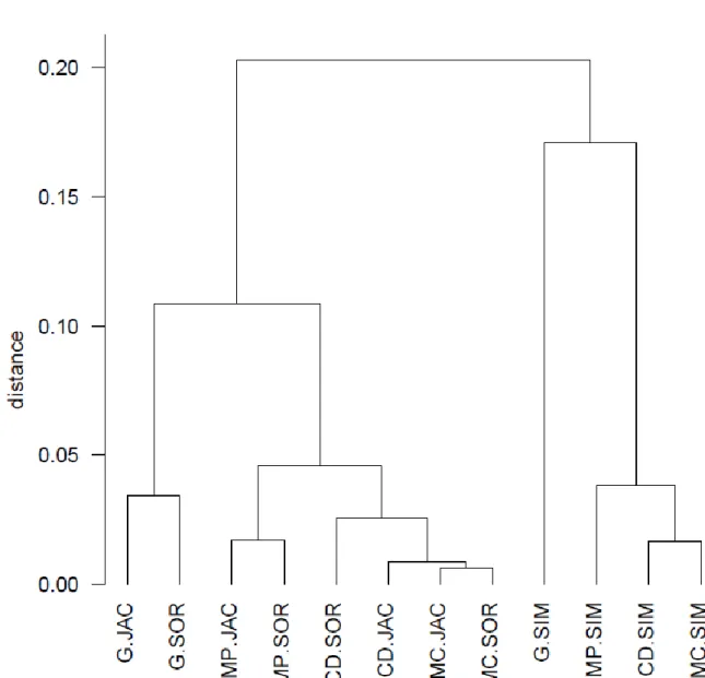
The dendrogram (Fig. 1) shows that methods belonging to the Simpson family constitute one 265
group, separated from the methods of the Jaccard and Sørensen families grouped in the 266
other. Within the latter, general coefficients are well-separated and grouping is more 267
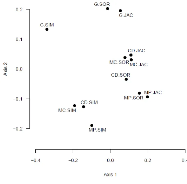
strongly influenced by the choice of approach than by the family (Fig. 1). The PCoA 268
ordination of the methodologies (Fig. 2) supports these conclusions. The first axis separates 269
the Simpson family from the Jaccard and Sørensen families, while the second separates the 270
general approach from the others. Since these axes account for 44% and 29% of the total 271
variance, respectively, we can conclude that choice between families had stronger impact on 272
the results than another decision between the general overlap approach and the others.
273 274
7.3 Artificial data 2 275
276
Artificial data set 1 allowed examining all theoretical possibilities in a matrix with very few 277
sites and species. To obtain a more realistic picture on the relationships among measures, 278
we generated a second artificial data set that is closer to actual community data. We 279
produced 150 sets of 10 sites by 10 species incidence matrices, in which the probability of 280
the occurrence of a species in a particular site was 0.5. We removed degenerate matrices 281
(i.e. those with zero row or column totals) and used the first 100 matrices. We followed the 282
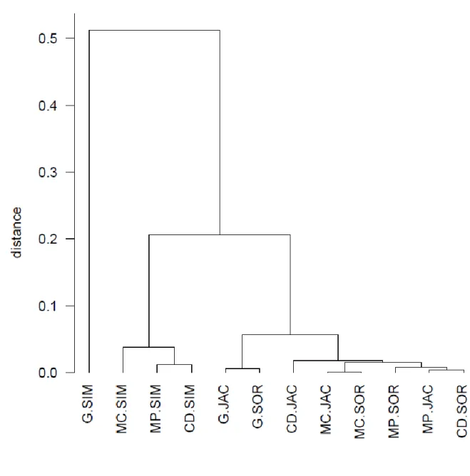
multivariate exploration procedure applied to artificial data set 1. The dendrogram (Fig. 3) 283
shows that methods belonging to the Simpson family form one group, and methods 284
belonging to the Jaccard and Sørensen families appear in another. Within the second group, 285
general coefficients are well-separated. The difference between Figs. 1 and 3 are that Fig. 3 286
shows larger distances among some groups of methods (the maximum distance is larger 287
than 0.5) and at the same time smaller distances among similar methods (the behavior of 288
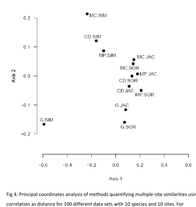
MC.JAC and MCSOR is similar). The PCoA ordination of the measures (Fig. 4) resulted in 289
much the same conclusions. The separation of the G.SIM from the other methods is clear.
290
On the first axis the Simpson family is distinguished from the Jaccard and Sørensen families, 291
while the second axis separates the general approach from the others. Since these axes 292
account for 68% and 16% of the total variance, respectively, we can conclude that choice 293
between families had stronger impact on the results than the decision between the general 294
overlap approach and the others. We may thus derive the final conclusion from clustering 295
and ordination that the general indices, especially those belonging to the Simpson family, 296
present a rather unique way of calculating multiple-site similarities.
297 298
7.4 Actual data set 299
300
Rey (1981) examined the recolonization of islets by arthropods after defaunization by 301
insecticides. The fauna was recorded every week for more than a year; we took the data 302
from the 10th, 13th, 20th and 53rd weeks after treatment. These four data matrices, 303
published in Atmar & Patterson (1995) contain 6 sites and 25, 27, 33 and 33 species, 304
respectively. An analysis equivalent to the mean pairwise Jaccard method indicated a 305
monotonic increase of similarity over the study period (Podani & Schmera 2011).
306 307
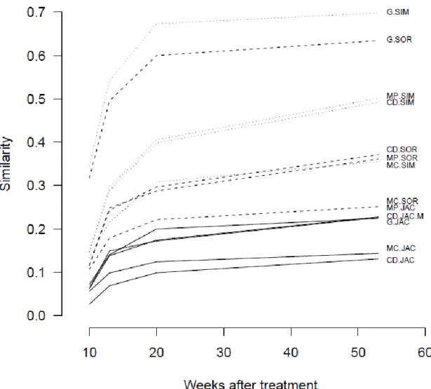
We found that all methods compared here indicate a monotonically increasing similarity 308
over time (Fig. 5). Nonetheless, the methods show considerable differences regarding the 309
multiple site similarity in the four assemblages. For instance, in week 53, the Jaccard family 310
co-diversity index (CD.JAC) yields a similarity value of 0.131, while the Simpson family 311
general index (G.SIM) produces 0.698. This suggests that selection of the methodology (i.e.
312
the choice of the family together with the approach) has significant impact on our inference 313
about community pattern (here similarity). It is important to note that the traditionally used 314
mean of pairwise indices (here abbreviated as mean pairwise method) and the other "true"
315
multiple-site indices produced very different results, suggesting that the pairwise and 316
multiple-site measures are complementary.
317 318 319
8. Conclusions 320
321
We emphasized that understanding and interpreting the multiple-site community patterns 322
pose relevant methodological issues of contemporary ecology and biogeography. Our review 323
demonstrated that a wide variety of methods have been available for quantifying multiple- 324
site resemblance patterns. To help the ecologist navigating among them, we suggested a 325
classification of methodology. Accordingly, a method is a combination of an index family and 326
an approach. Analyses of simulated and actual data sets revealed that inference drawn on 327
community pattern strongly depends on the applied method: multiple-site incidence 328
coefficients quantify different facets of multiple-site community patterns. In particular, we 329
found that the impact of choosing from original pairwise index families was stronger on 330
quantifying multiple-site resemblance patterns than the impact of selecting different 331
approaches. Thus, any methodology used for studying multiple-site community patterns 332
should be carefully evaluated before use.
333 334 335
Acknowledgements 336
337
We thank Hector Arita and Carlo Ricotta for their constructive comments on an earlier draft 338
of the manuscript. This research was supported by GINOP-2.3.2-15-2016-00019 project.
339 340 341
References 342
343
Arita, H.T. (2017) Multisite and multispecies measures of overlap, co-occurrence, and co- 344
diversity. Ecography, 40: 709-718.
345
Arita, H.T, Christen, J.A., Rodriguez, P. & Soberon, J. (2008) Species diversity and distribution 346
in presence-absence matrices: mathematical relationships and biological implications.
347
The American Naturalist, 172, 519-532.
348
Arita, H.T, Christen, J.A., Rodriguez, P. & Soberon, J. (2012) The presence-absence matrix 349
reloaded: the use and interpretation of range-diversity plots. Global Ecology and 350
Biogeography, 21, 282-292.
351
Atmar, W & Patterson, B.D. (1995) The nestedness temperature calculator: a visual basic 352
program, including 294 presence-absence matrices. AICS Research Inc., Univ. Park, NM 353
and The Field Museum, Chicago, IL 354
Baselga, A. (2010) Partitioning the turnover and nestedness components of beta diversity.
355
Global Ecology and Biogeography, 19, 134-143.
356
Baselga, A. (2012) The relationship between species replacement, dissimilarity derived from 357
nestedness and nestedness. Global Ecology and Biogeography, 21, 1223-1232.
358
Baselga, A. (2013) Multiple site dissimilarity quantifies compositional heterogeneity among 359
several sites, while average pairwise dissimilarity might be misleading. Ecography, 36, 360
124-128.
361
Baselga, A., Jiménez-Valverde, A. & Niccolini, G. (2007) A multiple-site similarity measures 362
independent of richness. Biology Letters, 3, 642-645.
363
Baselga, A. & Leprieur, F. (2015) Comparing methods to separate components of beta 364
diversity. Methods in Ecology and Evolution, 6, 1069-1079.
365
Baselga, A., Orme, D., Villeger, S., de Bortoli, J & Leprieur, F. (2013) betapart: Partitioning 366
beta diversity into turnover and nestedness components. R package version 367
1.3.http://CRAN.R-project.org/package=betapart 368
Bell, G. (2005) The co-distribution of species in relation to the neutral theory of community 369
ecology. Ecology, 86, 1757-1770.
370
Cardoso, P., Rigal, F., Carvalho, J.C., Fortelius, M., Borges, P.A.V., Podani, J. & Schmera, D.
371
(2014) Partitioning taxon, phylogenetic and functional beta diversity into replacement 372
and richness difference components. Journal of Biogeography, 41, 749-761.
373
Carvalho J.C., Cardoso, P., Borges, P.A.V., Schmera, D. & Podani, J (2013) Measuring fractions 374
of beta diversity and their relationships to nestedness: a theoretical and empirical 375
comparison of novel approaches. Oikos, 122, 825-834.
376
Chao, A., Chiu, C.C. & Hsieh, T.C. (2012) Proposing resolution to debates on diversity 377
partitioning. Ecology, 93, 2037-2051.
378
Chen, Y. (2016) Partitioning multiple-site tree-like beta diversity into turnover and 379
nestedness components without pairwise comparisons. Ecological Indicators, 61, 413- 380
417.
381
Diserud, O.H. & Ødegaard, F. (2007) A multiple-site similarity measure. Biology Letters, 3, 20- 382
22.
383
Gotelli, N.J. & Chao, A. (2013) Measuring and estimating species richness, species diversity, 384
and biotic similarity from sampling data. Encyclopedia of Biodiversity, vol. 5, pp. 195- 385
211.
386
Jaccard, P. (1912) The distribution of the flora in the alpine zone. New Phytologist, 11, 37-50.
387
Jost, L., Chao, A. & Chazdon R.R. (2011) Compositional similarity and β (beta) diversity. In 388
Magurran A.E. & McGill B.J. (eds) Biological diversity. Frontiers in measurement and 389
assessment. Oxford University Press, pp. 66-84.
390
Koch, L.F. (1957) Index of biotic dispersity. Ecology, 38, 145-148.
391
Koleff, P., Gaston, K.J. & Lennon, J.L. (2003) Measuring beta diversity for presence-absence 392
data. Journal of Animal Ecology, 72, 367-382.
393
Legendre, P. (2014) Interpreting the replacement and richness difference components of 394
beta diversity. Global Ecology and Biogeography, 23, 1324-1334.
395
Legendre, P. & De Cáceres M. (2013) Beta diversity as the variance of community data:
396
dissimilarity coefficients and partitioning. Ecology Letters, 16, 951-963.
397
MacKenzie D.I., Bailey L.L & Nichols J.D. (2004) Investigating species co-occurrence patterns 398
when species are detected imperfectly. Journal of Animal Ecology, 73, 546-555.
399
Orlóci, L. 1972. On objective functions of phytosociological resemblance. American Midland 400
Naturalist, 88, 28-55.
401
Podani, J. (2001) SYN-TAX 2000. Computer programs for data analysis in ecology and 402
systematics. Scientia, Budapest.
403
Podani, J. & Schmera, D. (2011) A new conceptual and methodological framework for 404
exploring and explaining pattern in presence-absence data. Oikos, 120, 1625-1638.
405
Podani, J & Schmera, D. (2016) Once again on the components of pairwise beta diversity.
406
Ecological Informatics, 32, 63-68.
407
Pollock L.J., Tingley R.,Morris W.K., Golding N., O’Hara R.B., Parris K.M., Vesk P.A. &
408
McCarthy M.A. (2014) Understanding co-occurrence by modelling species 409
simultaneously with a Joint Species Distribution Model (JSDM). Methods in Ecology 410
and Evolution, 5, 397–406 411
R Core Team (2015). R: A language and environment for statistical computing. R Foundation 412
for Statistical Computing, Vienna, Austria. URL https://www.R-project.org/.
413
Rey, J.R. (1981) Ecological biogeography of arthropods on Spartina islands in northwestern 414
Florida. Ecological Monographs, 51, 237-265.
415
Ricotta, C. & Pavoine, S. (2015) A multiple-site dissimilarity measure for species 416
presence/absence data and its relationship with nestedness and turnover. Ecological 417
Indicators, 54, 203-206.
418
Schmera D (2017) On the operative use of community overlap in analyzing incidence data.
419
Community Ecology, 18, 117-119.
420
Simpson, G.G. (1943) Mammals and the nature of continents. American Journal of Science, 421
241, 1-31.
422
Sørensen, T.A. (1948) A method of establishing groups of equal amplitude in plant sociology 423
based on similarity of species content, and its application to analyses of the vegetation 424
on Danish commons. Kongelige Danske Viden- skabernes Selskabs Biologiske Skrifter, 425
5, 1–34.
426
Trejo-Barocio, P. & Arita, H.T. (2013) The co-occurrence of species and the co-diversity of 427
sites in neutral models of biodiversity. Plos One, 8, e79918.
428
Warnes GR, Bolker B, Lumley T (2014) gtools: Various R programming tools. R package 429
version 3.4.1. http://CRAN.R-project.org/package=gtools 430
Whittaker, R.H. (1960) Vegetation of the Siskiyou Mountains, Oregon and California.
431
Ecological Monographs, 30, 279-338.
432
Whittaker, R.H. (1972) Evolution and measurement of species diversity. Taxon, 21, 213-251.
433 434
TABLES 435
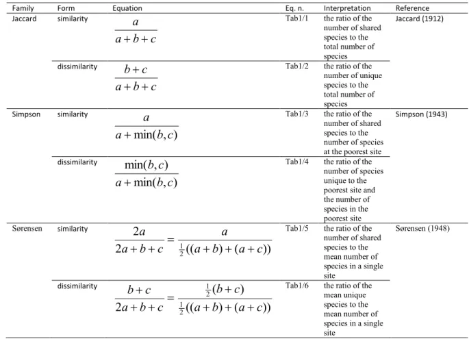
Table 1. The most important properties of three well known pairwise resemblance coefficients 436
Family Form Equation Eq. n. Interpretation Reference
Jaccard similarity
c b a
a
Tab1/1 the ratio of the number of shared species to the total number of species
Jaccard (1912)
dissimilarity
c b a
c b
Tab1/2 the ratio of the
number of unique species to the total number of species Simpson similarity
) , min(b c a
a
Tab1/3 the ratio of the number of shared species to the number of species at the poorest site
Simpson (1943)
dissimilarity
) , min(
) , min(
c b a
c b
Tab1/4 the ratio of the number of species unique to the poorest site and the number of species in the poorest site Sørensen similarity
)) ( ) ((
2 2
21 a b a c
a c
b a
a
Tab1/5 the ratio of the number of shared species to the mean number of species in a single site
Sørensen (1948)
dissimilarity
)) ( ) ((
) (
2 21
2 1
c a b a
c b c
b a
c b
Tab1/6 the ratio of the
mean unique species to the mean number of species in a single site
437 438
439
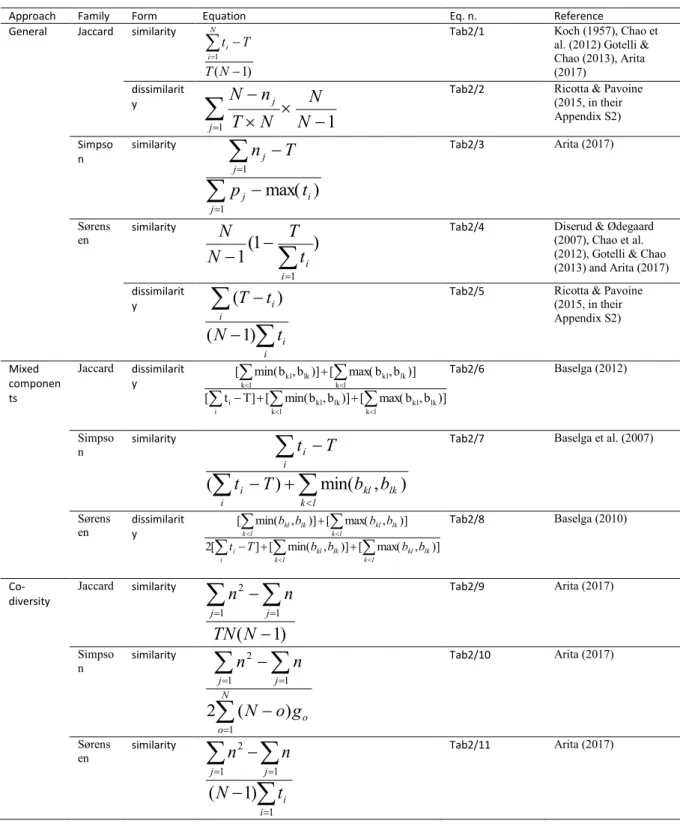
Table 2: Overview of multiple site resemblance coefficients (N: number of sites, T: total number of 440
species, ti: number of species at site i, nj: number of sites where species j occurs, o: rank of a species 441
richness value in the order from the smallest to the largest values, go: the frequency of sites with 442
species richness of rank o, bkl: number of species unique to site k in pairwise comparison with site l, 443
blk: number of species unique to site l in pairwise comparison with site k).
444
Approach Family Form Equation Eq. n. Reference
General Jaccard similarity
) 1 (
1
N T
T t
N i
i
Tab2/1 Koch (1957), Chao et al. (2012) Gotelli &
Chao (2013), Arita (2017)
dissimilarit
y
1 1
j
j
N N N T
n
N Tab2/2 Ricotta & Pavoine
(2015, in their Appendix S2) Simpso
n
similarity
1 1
) max(
j
i j
j j
t p
T
n Tab2/3 Arita (2017)
Sørens
en similarity
) 1
1(
1
i
ti
T N
N Tab2/4 Diserud & Ødegaard
(2007), Chao et al.
(2012), Gotelli & Chao (2013) and Arita (2017) dissimilarit
y
i i i
i
t N
t T
) 1 (
)
( Tab2/5 Ricotta & Pavoine
(2015, in their Appendix S2)
Mixed componen ts
Jaccard dissimilarit
y
i kl kl
lk kl lk
kl i
l
k kl
lk kl lk
kl
] ) b , b max(
[ )]
b , b min(
[ ] T t [
] ) b , b max(
[ )]
b , b min(
[ Tab2/6 Baselga (2012)
Simpso
n similarity
i k l
lk kl i
i i
b b T
t
T t
) , min(
) (
Tab2/7 Baselga et al. (2007)
Sørens
en dissimilarit
y
i kl kl
lk kl lk
kl i
l
k kl
lk kl lk
kl
b b b
b T
t
b b b
b
] ) , max(
[ )]
, min(
[ ] [ 2
] ) , max(
[ )]
, min(
[ Tab2/8 Baselga (2010)
Co- diversity
Jaccard similarity
) 1 (
1 1
2
N TN
n n
j j
Tab2/9 Arita (2017)
Simpso
n similarity
N o
o
j j
g o N
n n
1
1 1
2
) ( 2
Tab2/10 Arita (2017)
Sørens
en similarity
1 1 1
2
) 1 (
i i j j
t N
n
n Tab2/11 Arita (2017)
445 446 447
448
FIGURES 449
450
451
Fig. 1: UPGMA clustering of methods quantifying multiple-site similarities using 1 – 452
correlation as distance for 41,503 different data sets with 4 species and 4 sites.
453
Abbreviations include the combination of an approach and a family, where one or two 454
letters denote an approach (MP: mean pairwise, G: general, MC: mixed component and CO:
455
co-diversity) and after a dot three letters denote a family (JAC: Jaccard, SIM: Simpson and 456
SOR: Sørensen).
457
458
459
Fig 2: Principal coordinates analysis of methods quantifying multiple-site similarities using 1 460
– correlation as distance for 41,503 different data sets with 4 species and 4 sites. For 461
abbreviations, see caption to Fig. 1.
462 463
464
Fig. 3: UPGMA clustering of methods quantifying multiple-site similarities using 1 – 465
correlation as distance for 100 different data sets with 10 species and 10 sites. For 466
abbreviations, see caption to Fig. 1.
467 468
469
Fig 4: Principal coordinates analysis of methods quantifying multiple-site similarities using 1- 470
correlation as distance for 100 different data sets with 10 species and 10 sites. For 471
abbreviations, see caption to Fig. 1.
472 473 474
475
Fig. 5: Change of community similarity over time (in weeks) depicted by 13 multiple-site 476
similarity indices. For clarity, data points are connected. For abbreviations, see caption to 477
Fig. 1.
478 479