Ecological and evolutionary dynamics of interconnectedness and modularity

(1)

Ecological and evolutionary dynamics of interconnectedness and modularity

Jan M. Nordbotten^a,b, Simon A. Levin^c, Eörs Szathmáry^d,e,f, and Nils C. Stenseth^g,1

aDepartment of Mathematics, University of Bergen, N-5020 Bergen, Norway;^bDepartment of Civil and Environmental Engineering, Princeton University, Princeton, NJ 08544;^cDepartment of Ecology and Evolutionary Biology, Princeton University, Princeton, NJ 08544;^dParmenides Center for the Conceptual Foundations of Science, D-82049 Pullach, Germany;^eMTA-ELTE (Hungarian Academy of Sciences—Eötvös University), Theoretical Biology and Evolutionary Ecology Research Group, Department of Plant Systematics, Ecology and Theoretical Biology, Eötvös University, Budapest, H-1117 Hungary;^fEvolutionary Systems Research Group, MTA (Hungarian Academy of Sciences) Ecological Research Centre, Tihany, H-8237 Hungary; and^gCentre for Ecological and Evolutionary Synthesis (CEES), Department of Biosciences, University of Oslo, N-0316 Oslo, Norway

Contributed by Nils C. Stenseth, December 1, 2017 (sent for review September 12, 2017; reviewed by David C. Krakauer and Günter P. Wagner) In this contribution, we develop a theoretical framework for linking

microprocesses (i.e., population dynamics and evolution through natural selection) with macrophenomena (such as interconnectedness and modularity within an ecological system). This is achieved by de- veloping a measure of interconnectedness for population distributions defined on a trait space (generalizing the notion of modularity on graphs), in combination with an evolution equation for the population distribution. With this contribution, we provide a platform for understanding under what environmental, ecological, and evolutionary conditions ecosystems evolve toward being more or less modular.

A major contribution of this work is that we are able to decompose the overall driver of changes at the macro level (such as interconnectedness) into three components: (i) ecologically driven change, (ii) evolutionarily driven change, and (iii) environmentally driven change.

microevolution

|

population biology

|

macroecological patterns

|

macroevolutionary patterns

|

mathematical modeling

I

n evolutionary biology, as in other branches of science, there is a gap between macroscopic patterns and microscopic dynamics, raising the challenge of relating microevolutionary and macroevolutionary perspectives. Here we aim at contributing toward bridging this gap by using a population-based microevolutionary model (where genetic variation modeled as a diffusion process leads to microevolution) to deduce the long-term dynamics of macroecological features of ecological systems. Specif- ically, we aim at contributing toward the understanding of how macroecological features change over time as a result of population−biological processes. As our focal macroecological fea- ture, we have chosen the issue of interconnectedness, including a generalization of the notion of network modularity (1–3). Modu- larity is an important concept in evolutionary biology (4). How- ever, an understanding is lacking of when and how it emerges from ecoevolutionary processes. Essentially, we provide a platform for understanding under what environmental, ecological, and evolutionary conditions ecosystems evolve toward being more or less modular; see also Lorenz et al. (5) for an excellent and comple- mentary approach to the emergence and evolution of modularity.

We focus on interconnectedness, that is, how species within an ecosystem relate to each other, both qualitatively (i.e., competitive, trophic, etc.) and quantitatively (i.e., the strength of the ecological interaction). The concept of interconnectedness bears resemblance to notions of alpha, beta, and gamma diversity in community ecology (6), but expressed in terms of nearness in trait space rather than geographical space. Our approach is linked with the tradition of investigating complexity and stability in ecosystems (7, 8). That topic has traditionally ignored evolutionary processes, focusing just on the ecological dynamics [see, e.g., refs. 9–11]; it leaves open the fundamental question of how evolution will shape emergent properties like modularity and robustness. We address this lack through the inclusion of a genetic operator. We concretize our study of interconnectedness by addressing the overall question of how ecological and microevolutionary processes together impact the macroscopic measures of structure of the ecosystems arising from our model. A

refinement of this inquiry is to look for compartmentalization (i.e., modularity) in ecosystems. In food webs, for example, compartments (which are subgroups of taxa with many strong interactions in each subgroup and few weak interactions among them) have been empirically identified and revealed to increase stability (12–15). Asking questions regarding how interconnectedness changes over time corresponds to querying how the structure of the ecological interactions changes over time, on both short and long time scales.

A main contribution of this study is the partitioning of the driving forces behind the evolutionary change of interconnectedness into three components: (i) ecologically driven change, (ii) evolutionarily driven change, and (iii) environmentally driven change. This partitioning is inspired by the foundational contribution of Fisher (16), who showed that the variance of a trait can be partitioned into variance due to the environment and variance due to genetic components, including additive genetic effects, dominance effects, and epistasis.

We first provide the basic dynamic model, a mathematical definition of interconnectedness and modularity, followed by a partitioning into three components of drivers. These results are then discussed specifically with respect to our formulations, as well as with respect to the more general related literature.

Sources of Change in Macroevolutionary Processes and Patterns Our overall purpose is to provide a theoretical framework for linking measures of macroevolutionary processes and patterns to microevolutionary processes. For this purpose, we will use a set of measures of interconnectedness as macroscopic descriptors. Specifically, we will aim to achieve an understanding of how interconnectedness

Significance

This work contains two major theoretical contributions: Firstly, we define a general set of measures, referred to as interconnectedness, which generalizes and combines classical notions of diversity and modularity. Secondly, we analyze the temporal evolution of interconnectedness based on a microscale model of ecoevolutionary dynamics. This we do by providing a platform for understanding how and why macroecological phenomena change over long time scales. Such a platform allows us to show how the drivers of the dynamics of macroecological descriptors, such as interconnectedness, can be partitioned into three components: (i) ecologically driven change, (ii) evolutionarily driven change, and (iii) environmentally driven change.

Author contributions: J.M.N. and N.C.S. designed research; J.M.N. and N.C.S. performed research; and J.M.N., S.A.L., E.S., and N.C.S. wrote the paper.

Reviewers: D.C.K., Santa Fe Institute; and G.P.W., Yale University.

The authors declare no conflict of interest.

This open access article is distributed underCreative Commons Attribution-NonCommercial- NoDerivatives License 4.0 (CC BY-NC-ND).

1To whom correspondence should be addressed. Email: n.c.stenseth@ibv.uio.no.

This article contains supporting information online atwww.pnas.org/lookup/suppl/doi:10.

1073/pnas.1716078115/-/DCSupplemental.

(2)

depends on, and changes in response to, ecological processes and evolution within populations (i.e., microevolution). Within this context, we carefully assess the concept of interconnectedness, and provide an operational definition of this term. Thereafter, we introduce a general ecoevolutionary model and discuss the microevolutionary and ecological drivers of system-level changes in interconnectedness. In framing our results in terms of continuous distributions, we are basically assuming that the population is infin- ite, and neglecting genetic drift due to demographic stochasticity.

Ecological Interaction and Evolution. To prescribe a reasonably general model for ecological interaction and evolution, we introduce the concept of a high-dimensional spaceΩ, where the di- mensions correspond not just to observable traits but, in a broad sense, to all traits of relevance (17). Specifically, we considerkin- dependent traits (or trait families), which define the characteristics of the population of interest. We consider that all observables are continuous parameters (e.g., length, height, strength), although the case of discrete observables (number of legs, spots, fins, etc.) can be accommodated. As such, any combination of phenotypes can be represented by a position vectorx∈Ω, where Ω⊆R^k. Given this representation, a community [consisting of population(s) of a single or multiple species] can be represented as a density function overΩ;

i.e., any community is equivalent to a positive functionnðx,tÞ, wheret is a time variable. We allow the density functionnto take continuous values, indicating that the expected population sizes are considered, and note that nintegrated over Ω corresponds to the total population size. When necessary, individual species can be identified as peaks in the distributionn, while the phenotypic variation within a species will correspond to the spread ofnaround the peak corre- sponding to that species (18) (see Supporting Information for an example of this). We note that, while this approach, in principle, requires a high-dimensional space Ω, empirical evidence suggests that, in practice, many ecosystems align themselves on relatively low- dimensional submanifolds (19).

We limit the discussion to a community that can be considered to have negligible physical extent; thus our position vector only relates to trait space. Taking this into consideration, the term

“total population density” refers to the summed density of all individuals in the community. In this case, a fairly general model for ecological interaction and evolution can be stated as

∂

∂tnðx,tÞ=nðx,tÞAfng+∇·ðgðx,tÞ∇nðx,tÞÞ. [1]

Eq. 1 thus relates the rate of change of the total population density to ecological interactions as represented by the growth/

decay rateA(which is dependent on the current system state), and to intergenerational phenotypic (diffusive) change via a second-order differential operator, whereghas the interpretation of phenotypic dispersion per time. As such, Eq.1is a generalization of reaction−diffusion type equations, and includes common models in ecology and evolution as subsets (see, e.g., refs.

20–22; for a more detailed discussion, see refs. 17 and 23).

In Eq.1, the functionnðx,tÞas well as the evolvabilitygðx,tÞare, in general, functions of both phenotype position and timeðx,tÞ.

Similarly, the functionalAwill also, in general, be dependent on space and time, and takes all current values ofnas argument. Eq.1 must be complemented with boundary conditions; we will herein only consider the case where the parameter spaceΩeither is pe- riodic or is large enough that the solutionnðx,tÞcan be considered to have compact support [in which case, bothnðx,tÞand its de- rivatives are zero for allxon the boundary ofΩ]. We have chosen to consider a normal diffusive operator in Eq.1. The results that follow can be further generalized to diffusive differential operators of fractional order, equivalent to distributions with so-called fat tails. Our use of a diffusion operator differs from the standard diffusion in population genetics, namely, the diffusion of types due to finite populations, whose strength decays to zero as types hit the boundary of frequency space.

The time dependence of the parameter functions reflects changes in environmental conditions. As an example, we can consider a case

where environmental conditions are given by a set of parameter functions, which we denote by EðtÞ. Here the interpretation is that environmental conditions include everything external to the population in consideration, be they abiotic or biotic factors. We can then make the dependence of A explicitly dependent on the external conditions, that is to say,Afng=Afn,EðtÞg.

The formalism stated in Eq. 1allows for any prescribed environmental conditions. A special case is where the external conditions themselves satisfy a separate evolution equation (see, e.g., work by refs. 24 and 25), such as, for example,

∂

∂tEðtÞ=F ðE,nÞ. [2]

Thus, we have a coupled system, where the population influences the external conditions throughF, while the external conditions evolve in time, and provide the parameters for the population dynamics ofnðx,tÞ; cf. also ref. 26.

We understandnin a probabilistic sense, such that it represents a continuous density function (rather than a precise discrete accounting of individuals). Thus, the second term of Eq.1 represents, in a probabilistic sense, the spread in phenotype space associated with intergenerational variability due to mutations during inheritance. The parametergthus has the interpretation of trait variability per generation, expressed in continuous time. Evo- lution arises as the ecological interactions encoded inAprovide favorable circumstances for certain parts of the variability introduced through the diffusive term.

The incremental impact functionαðx,x^’;nÞof any individual with traitsx’on an individual with traitsx(given a populationn) is represented by the derivative ofA, which we denote by

α=DA. [3]

The gradientDA(technically the Fréchet derivative) is the suitable generalization of the gradient operator to functionals. For example, negative values of both αðx,x′;nÞ and αðx,x′;nÞ correspond to competition between individuals (or species) with traitsxandx′, while positive values represent mutualism. When the signs ofαðx,x′;nÞand αðx,x′;nÞare opposite, exploiter−victim dynamics are involved.

The special case whereAis linear leads toαðx,x′Þ, independent of the current staten, and was studied in ref. 17. In this linear case, the functional can be expressed in terms of the integral operator,

Afng=rðxÞ+ Z

Ω

αðx,x′Þnðx′Þdx′. [4]

By considering here a more general model, we thus allow for interspecies interactionsα, which depend on the species composition itself.

Our approach may be linked with the tradition of investigating complexity and stability in ecosystems (7, 8, 25), a topic traditionally restricted to the ecological time scale. We go further because of the inclusion of the genetic operator. Our model allows us to explore the species and interactions that may coexist, as well as the ecological circumstances that underpin this coexistence. This can be modified to look at compartmentalization (modularity) in ecosystems. In food webs, for example, compartments (subgroups of taxa with many strong interactions in each subgroup and few weak interactions among them) have been empirically identified and revealed to increase stability (12–14). Our model is furthermore connected to the adaptive dynamics approach, in that Eq.1can be seen as the con- tinuum limit of the stochastic processes from which the so-called canonical equation of adaptive dynamics is derived (22). In the special case of well-defined and distinct species with small mutation rates (when traits can be approximated as normally distributed), Eq.

1is an equivalent formulation of the canonical equation.

Measures of Interconnectedness and Modularity. Interconnected- ness and the closely related concept of modularity are examples of widely used concepts that address structural properties of communities and ecosystems (27–29).

Our intention is to consider a family of related interconnectedness measures, which not only reflect the number and abundance of species within a system but also the variability within each

EVOLUTIONAPPLIED MATHEMATICS

(3)

species. It is therefore not sufficient to consider measures based solely on counting species (30); we also need to incorporate measures of both interspecies and intraspecies variability. Our concept of interconnectedness is a functional one, in that we aim for a metric that not only evaluates the individuals present in a population but also honors their interactions in the ecological system. To discuss interconnectedness in a macroevolutionary setting, it is imperative to have definitions that not only capture the current state of the system but also are sensible in the face of speciation and extinction. It follows that a measure in this context must honor both interspecies and intraspecies variability.

With this motivation, we start by considering the total population size, defined as a time-dependent quantity,

NðtÞ= Z

Ω

nðx,tÞdx. [5]

To define a measure of interconnectedness (and later modularity), we need two concepts. First, we consider the distance between two individuals with phenotypes xand x′in the space of observables, which we define asdðx,x′Þ. As a distance measure, we require that it satisfies the natural conditions that it is symmetric and positive [dðx,x′Þ=dðx′,xÞ>0 for x≠x′] and that dðx,x′Þ=0 if and only ifx=x′; however, we will, at present, not specify it further. Secondly, we consider the interactions within the species, and we define the interaction strengthϕðx,x^’;t,nÞas a measure of the impact (or expected impact) of an individual with traits x′ as observed by an individual with traits x. The (parametric) dependence of ϕ on tand nimplies that the interaction strengths can depend both on external time-evolving factors and on the population structure itself. We will return to suggest a precise definition ofϕlater.

A secondary consideration is that it is useful, from a modeling perspective, if measures of interconnectedness and modularity have information content not only as measurements of the state of the system but also as variables internal to the system. To this end, we introduce the concept of “observed interconnectedness” Hxfng.

Here, and in the remainder of this section, we will suppress the dependence on t, with the understanding that since n is time- dependent, all definitions depending on n are also, in general, time-dependent. More precisely, we define byHxfngthe connec- tions within the system as seen from an individual with phenotype positionx. To propose a candidate forHxfng, we take an axiomatic approach, and suggest that the following properties are desirable for a measure of interconnectedness: (i) The observed interconnectedness Hx must be positive, i.e.,Hxfng≥0 for all admissiblen.

(ii) We defineHxto be zero for homogeneous populations where all members have identical traits, i.e.,Hxfng=0 whennðx′Þ=δðx′−xÞ;

a Dirac delta distribution centered atx′. (iii) From an operational perspective, an individual cannot observe any interconnectedness associated with species it does not have any interaction with; thus, for two populations n1 and n2, the observed interconnectedness Hxfn1+n2g=Hxfn1gif the observer atxhas no interaction with members of populationn2. (iv) The observed interconnectedness cannot decrease with the addition of new individuals to the population, i.e.,Hxfn1+n2g≥Hxfn1g.

To discuss the difference in structure between differences in traits and strength of interactions, we will use the additional property that (v) for a population composed of a single species, interconnectedness should not decrease when the variance of traits increases; that is, if we define a normal distribution with variance e as δeðxÞ, then Hxfδeg should be a continuous and monotone function of the variance of traits.

When omitting this property, and thus neglecting the differences in traits, we can recover standard measures of diversity as special instances of interconnectedness. This is detailed in Supporting Information.

The following functional form is perhaps the simplest that satisfies all of the above relationships, while retaining a reasonable generality:

Hxfng=1 N

Z

Ω

nðx′Þhðx,x′Þ dx′, [6]

where the observed interconnectedness kernel is given by the product of interaction and distance, hðx,x′Þ=dðx,x′Þϕðx,x′Þ.

Observed interconnectedness as defined in Eq. 6can be interpreted in several ways, including as the observed population (fromx) relative to the total population. Secondly, if we consider ϕ=1, we see that the observed interconnectedness measures the total distance (in trait space) of the population fromx. Thirdly, we take dðx,x′Þ=1 for all x≠x′; we obtain the alternative interpretation ofHxfngas the total influence of the ecosystem on an observer atx. As such, we understand thatHxfng, in principle, represents a family of interconnectedness measures of the population. This third interpretation also motivates the dual concept of the“imposed interconnectedness,” in other words, to what extent an individual at x interacts with the existing population n. The definition of the imposed interconnectedness is obtained by reversing the arguments in the kernel hðx,x^’Þ=hðx^’,xÞas

H^p_xfng=1 N

Z

Ω

nðx′Þhðx′,xÞ dx′. [7]

Taking again the special case of dðx,x′Þ=1 for all x≠x′, the functionalH_x^pfngcan be interpreted to measure the total impact of an individual atxon the populationnðxÞ.

We note that both the observed and imposed interconnectedness take on distinct values for each point in Ω, much in analogy to the coordination number or connectedness measures on graphs. From this analogy, we expect that the distributions of Hxfngand H_x^pfng will carry significant information about the system. Of particular importance are the total and weighted mean values of system interconnectedness. We define the total observed and imposed interconnectedness as

H_Ωfng= Z

Ω

Hxfngdx′ and H_Ω^pfng= Z

Ω

H_x^pfngdx′. [8]

For the (weighted) mean interconnectedness, we note that the mean observed interconnectedness must (by symmetry) equal the mean imposed interconnectedness, both defined as

Hfng=1 N

Z

Ω

nðxÞHxfngdx=1 N

Z

Ω

nðxÞH_x^pfngdx. [9]

From Eqs.7and9, we obtain, directly, the global interconnectedness measure,

Hfng= 1 N²

ZZ

Ω

nðxÞnðx′Þhðx,x′Þdx′dx. [10]

We will refer tohðx,x′Þas the interconnectedness kernel, which is symmetric and defined by

hðx,x′Þ=1 2

hðx,x′Þ+hðx,x′Þ

=1

2dðx,x′Þðϕðx,x′Þ+ϕðx′,xÞÞ.

From Eqs.10and11, we see that the interconnectedness mea-[11]

sureHreflects both the phenotypic distance between members of the population and the mutual interaction of individuals. If the population is a monotype, or if no individuals have any interaction, the interconnectedness will be zero.

While a much richer notion, the mean interconnectedness can nevertheless be related to measures of diversity such as the Shannon entropy or the Simpson measure by particular (de- generate) choices of dðx,x′Þandϕðx,x′Þ. We review these relationships inSupporting Information.

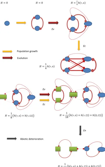
To increase the intuition for the interconnectedness measure, we illustrate the interconnectedness associated with some simple (yet typical) situations in Fig. 1; in Box 1, we further provide some gedanken examples illustrating our measure of interconnectedness.

(4)

The calculations used to obtain the illustrative values of interconnectedness are based on a discrete number of individuals (as opposed to the general formulation allowing for distribution of traits), as summarized inSupporting Information, in particular Eq.S3. This allows us to provide an interpretation of the interconnectedness kernelhðx,x′Þas the generalization of the adjacency matrix (or connectivity map) of a weighted directed network (or graph) to allow for continuous points, a so-called graphon (that is to say, the limiting case of a graph that is dense enough to be approximated as a continuous function). The observed and imposed interconnectedness functions thus generalize the row and column sums of the adjacency matrix, and the total interconnectedness is the sum of the entries.

Referring to Fig. 1, we note that, in general, the highest value of interconnectedness would be obtained by a population that is proportional to the eigenfunction ofhðx,x′Þwith the largest ei- genvalue. However, in most instances, eigenfunctions will take negative, positive, and possibly complex values, and thus the eigenfunctions of hðx,x′Þ provide only guidance to the general structure of the most interconnected population. From

Eq. 11, we note that dðx,x′Þ will tend to have eigenfunctions that favor populations with maximally dispersed traits, while ðϕðx,x′Þ+ϕðx′,xÞÞwill tend to have eigenfunctions that pick up the dominant interactions in the population. The total measure thus represents a compromise between trait variation and strong interactions.

Although we do not include classical genetics, we are considering hereditary phenotypes. However, if we had included genetics explicitly, we would have another component of interconnectedness. Two genotypes with the same phenotype can (i) have dif- ferent evolutionary potential or (ii) become distinct phenotypes when the biotic or the abiotic environment changes.

Interconnectedness as defined above is closely related to modularity (2) by using the interpretation introduced above of the interconnectedness kernel as the connectivity map of a graphon. More precisely, we consider the population nðxÞas a partition with respect to the space of all possible populations.

Then the generalization of Newman’s modularityQfrom graphs to continuous populations is given by

Qfng= 1 N²

ZZ

Ω

nðxÞnðx′Þqðx,x′Þdx′dx, [12]

whereqðx,x′Þis the deviation ofhðx,x′Þfrom its marginals,

qðx,x′Þ=hðx,x′Þ−RRhmðxÞhmðx′Þ

Ω

hðx,x′Þdx dx′, [13]

andhmis the marginal ofhðx,x′Þ,

hmðxÞ= Z

Ω

hðx,x′Þdx′. [14]

From the definitions of Qfng and Hfng, we obtain the relationship

Qfng=Hfng−

H_Ωfng+H_Ω^pfng2

4Hf1g . [15]

This relationship allows us to consider interconnectedness and modularity as interchangeable concepts.

Modularity has proven to be useful in investigating the sub- structure of populations. Thus, for any division of the population into two subpopulations, identified by a partition function sðxÞ taking values 1 and−1, the modularity of the division is given by QfsðxÞnðxÞg. Modular subpopulations can thus be identified by optimizingQfsðxÞnðxÞgover all possible partitions (31).

We obtain an explicit link between the interconnectedness measureHfngdefined in Eq.10and the ecoevolutionary system stated in Eqs.1–3by assuming that the interaction strengthϕis dependent on the impact functionα. To be concrete, we will take the interaction strength to be equal to the magnitude of the incremental impact function, such that

ϕðx,x′;nÞ=jαðx,x′;nÞj. [16]

The interconnectedness of an ecological population can then be determined by Eqs.3,10, and11.

Drivers of Change in Interconnectedness.A principal goal of our work is to determine the ecological and microevolutionary processes that drive changes in interconnectedness, and thereby also modularity. Taking Eq. 10 as a starting point, we can use the general ecoevolutionary model from Eq.1to evaluate the temporal change in interconnectedness as it responds to the ecological system. While we, in this section, deal with the mean interconnectednessHfngfor the community, the same approach applies directly to the observed and imposed interconnectedness HxfngandH_x^pfng. This leads to an expression of the form (see Supporting Informationfor details)

Fig. 1. Example of interconnectedness measure for a simple system. Circles/

squares and ovals/rectangles represent individuals with identical and similar positions in trait space, while the distance from circle/oval to square/rect- angle is large. The thickness of the lines indicates interaction strength ϕðx,x′Þ, while the total interconnectednessHof each system is expressed in terms of the interconnectedness kernels [e.g.,hð∘, 0Þ]. The arrows in the figure indicate a hypothetical temporal progression of the system.

(5)

dH

dt =Ecfng+Evfng+Enfng. [17]

In this sense, then, the interpretation of ref. 17 is inspired by Fisher’s original partitioning, here into moments, and applied to the concept of interconnectedness. We discuss these terms in detail below, but first note that Ecrepresents the change in interconnectedness due to ecological interactions, and is defined as

Ecfng= 2 N²

ZZ

Ω

AfngnðxÞnðx′Þ½hðx,x′,t;nÞ−Hdx′dx. [18]

This term thus represents the correlation between local imbal- ances in the interconnectedness kernel (the bracket term) and the population size and interaction.

Similarly,Evrepresents the change in interconnectedness due to evolutionary dynamics,

Evfng= 2 N²

ZZ

Ω

nðxÞnðx′Þ∇x·ðgðxÞ∇xhðx,x′,t;nÞÞdx′dx, [19]

which primarily is a reflection of the shape of the distance measure. Finally, En represents the impact of environmental change as

Enfng= 1 N²

ZZ

Ω

nðxÞnðx′Þd

dthðx,x′,t;nÞdx′dx. [20]

The three terms in Eq.17represent the main drivers for change in interconnectedness. For a system in equilibrium (i.e., stasis), Eq.20implies thatEnwill be zero, while we see from Eq.17that, while bothEcand Evmay be nonzero, they must be of equal magnitude with opposite signs. From this starting point, we can consider the causes of change in interconnectedness by considering the processes that influence the sign and magnitude of these three terms, and we discuss these in reverse order.

The environmental termEnrepresents the change in interconnectedness due to the local interconnectedness kernel h itself changing. This happens both due to external processes (both biotic and abiotic), which alter the interactions within an ecosystem, and due to the strength of interactions themselves, depending on the population structure. To make precise statements, consider the linear case, expressed in Eq.4, whereEnsolely represents external changes, sincehdoes not depend onnin this case. Thus, changes in En are understood through the correlation between the interconnectedness kernel and the system interactions defined in Eq.

16. Loosely speaking, we understand that environmental and population changes that lead to weaker interactions in the ecosystem (e.g., a relative abundance of resources, due to either external factors or a reduction in population) reduce the interconnectedness measure, while environmental conditions which lead to a strengthening of interactions lead to an increase in interconnectedness. This interpretation generalizes to weakly nonlinear systems. When, furthermore, the external conditions are constant and a linear model is considered (in the sense of Eq.4, as was the case in ref. 17),Enis zero.

In contrast, both Evand Ec directly reflect the population structure itself. In Supporting Information, we conclude thatEv will be positive with reasonable assumptions on the model, which confirms the intuitive notion that increased variability in traits during the process of reproduction leads to a general increase in interconnectedness.

To gain an understanding of the ecological driverEc, we will consider, for the moment, the setting of a linear ecological de- scription as given in Eq.4. Furthermore, we letrðxÞbe a positive constant andαðx,x′Þ≤0, so that the system is competitive. We provide the calculations for both this simplified case and the

general case of nonlinear systems, including competitive, mutualistic, and parasitic interactions, inSupporting Information.

In Supporting Information, we also show that, for the linear system, strong contributions to interconnectedness occur when, for two trait combinationsxandx′, (i) there is an abundance of individuals in the sense thatnðxÞandnðx′Þare both large, and (ii) the interactions are strong in the sense of αðx,x′Þ being large.

Furthermore, this trait combination will tend to decrease interconnectedness if, simultaneously, (iii) the interconnectedness kernel is relatively large, i.e.,hðx,x′Þ>H. By comparing conditions iiandiii, in light of the definition given in Eq.11, we understand that these two conditions will hold together if the distancedðx,x′Þ is large. This can be summarized as follows: Strong competitive interactions between dissimilar species will, in general, tend to reduce interconnectedness, while strong competitive interactions between similar species will increase interconnectedness. This last statement can be seen directly in terms of traditional concepts, and, in particular, to the ghost of competition past (32). Within this conceptualization, ecosystems and communities will tend to avoid strongly competing species, and thus reduce interconnectedness

Box 1: Gedanken Examples of Change in Interconnectedness

To provide a better intuitive understanding of the interconnectedness concept, we here provide some gedanken examples as to how some typical ecological and evolutionary changes might lead to changes in the degree of interconnectedness (additional examples may be found in ref. 5).

a. Speciation: During speciation, it is reasonable to assume that the interaction between the two new species is similar to the interaction within the original species. Thus, speciation may be thought of as two populations that are initially at the same phenotypic position, such thatd=0. During speciation, the two populations (=species) diverge, leading to an increase ind; as a result, the system interconnectedness will increase. An example of speciation involves Darwin’s finches on Galapagos (44).

b. Change in the overall environmental conditions: Envi- ronmental change may both increase and decrease interconnectedness through the impact on the interaction strengthϕ.

When, for instance, two ecosystems that have previously been physically separated merge, previously noninteracting species (ϕ=0) may interact (ϕ>0). This will naturally increase interconnectedness. The Bering land bridge is such an example (45).

c. Ecological dynamics: Ecological dynamics will continu- ously change the interconnectedness of a system. For example, an ecosystem with a very dominant species may be seen to have a relatively small interconnectedness, according to Eq.9 (assuming a relatively constant interaction strengthϕ). After the collapse of the dominant species (through internal or external processes), the resulting system will be more well- balanced, and will, in general, result in a higher degree of interconnectedness. The well-studied hare−lynx system may be seen as such an example of rapid change in relative population sizes (38, 39, 46).

d. Ghost of competition past: Connell (32) argues that measuring the apparent overlap of species in nature is a misleading way to measure the extent to which they compete.

Indeed, overlap may imply the absence of competition because species have been displaced to coexist. The degree of interconnectedness naturally differentiates these cases.

e. Autocatalytic sets and ecosystem functioning:Ecological systems develop syntrophy and other mutualistic interactions.

These interactions link species together into autocatalytic modules that are self-sustaining and interact perhaps more weakly with other modules, as suggested by Paine (15). Over evolutionary time, some linkages tighten, while others weaken.

The modularity of the system can be derived from the interconnectedness measures, as exposed in Eq.15.

(6)

if the competitors are dissimilar and (relatively speaking) increase interconnectedness when the competitors are similar. The slightly more nuanced interpretation for nonlinear systems is discussed in Supporting Information.

This also emphasizes the difference between measures of interconnectedness and diversity, wherein the latter generally do not include the concepts of trait distance, and, as such, do not capture the nuances associated with the similarity of species identified above.

Discussion and Conclusion

Our model relates to the tradition of Simpson (33), with regard to phenotypic and adaptive landscapes that are dynamically changing (see, e.g., refs. 22 and 34–36). These kinds of landscapes have been proposed to conceptually bridge microevolution and macroevolution (37). We submit that our model is a dynamical manifesta- tion of this goal, in that we account for the coevolutionarily and environmentally driven movement of the fitness optima.

In this contribution, we have emphasized the fundamental structure of interconnectedness and the ecological, evolutionary, and abiotic drivers for changes in this metric. The interconnectedness concept naturally applies to biological systems, in particular when interaction strengths have been determined. A particularly relevant example is the present-day vegetation−hare−lynx system of the Canadian boreal forest, for which interaction coefficients have been determined explicitly from time series analysis (38, 39).

To understand the changes in interconnectedness over time, longer records are needed, and analysis of paleontological data, based on assumptions of correlations between interaction and species overlap, provides a promising avenue (40); see also Box 1.

Interconnectedness and modularity are fundamental features of ecological systems, and are fundamental determinants of their

robustness in the face of endogenous and exogenous threats (41).

Simon (42) emphasized the importance of modularity through his parable of two watchmakers, and explored the dynamics of modular systems by demonstrating how they play out on multiple time scales (35) [in evolutionary biology, modularity plays a fundamental role, and arises naturally from microscopic forces (1, 3, 36)].

In this paper, we have developed a mathematical framework to explore the emergence of modularity. Inspired by Fisher’s foundational paper on components of variance, we partition the rate of change in modularity into the parts due to endogenous factors, specifically ecological and evolutionary dynamics, and those due to exogenous environmental changes. Such a partitioning may help us separate ecological and evolutionary drivers of variation of macroecological descriptors, not the least to differentiate between biotic and abiotic drivers of evolutionary dynamics (43). More generally, although we have focused on interconnectedness, the approach may be used to explore influences on other macroscopic descriptors.

ACKNOWLEDGMENTS.Jo Skeie Hermansen, Joshua Plotkin, Sergey Kryazhimskiy, Kjetil Lysne Voje, and Han Wang are all thanked for commenting upon an earlier version of this manuscript. Sari Cunningham is thanked for splendid linguistic and copy-editing work on the manuscript. Funding for this project was primarily covered by Centre for Ecological and Evolutionary Synthesis (core and Colloquium 4) funding and the Research Council of Norway (RCN) project, Red Queen coevolution in multispecies communities: Long-term evolutionary consequences of biotic and abiotic interactions (EVOQUE). In addition, S.A.L. acknowledges support through Simons Foundation Grant 395890 and Army Research Office Grant W911NF-14-1-0431. E.S. acknowledges support through the European Research Council [294332–EVOEVO (Evolution of Evolvable Systems)], GINOP-2.3.2-15-2016-00057, and Nemzeti Kutatási, Fejlesztési és Innovációs Hivatal (National Research, Development and Innovation Office) 119347.

1. Schlosser G, Wagner GP (2004)Modularity in Development and Evolution(Univ Chi- cago Press, Chicago).

2. Newman MEJ (2006) Modularity and community structure in networks.Proc Natl Acad Sci USA103:8577–8582.

3. Hartwell LH, Hopfield JJ, Leibler S, Murray AW (1999) From molecular to modular cell biology.Nature402:C47–C52.

4. Solé RV, Valverde S (2008) Spontaneous emergence of modularity in cellular networks.J R Soc Interface5:129–133.

5. Lorenz DM, Jeng A, Deem MW (2011) The emergence of modularity in biological systems.Phys Life Rev8:129–160.

6. Whittaker RH (1970)Communities and Ecosystems(Macmillan, New York).

7. Gardner MR, Ashby WR (1970) Connectance of large dynamic (cybernetic) systems:

Critical values for stability.Nature228:784.

8. May RM (1973) Stability and complexity in model ecosystems.Monogr Popul Biol6:

1–235.

9. May RM (1972) Will a large complex system be stable?Nature238:413–414.

10. Gilarranz LJ, Rayfield B, Liñán-Cembrano G, Bascompte J, Gonzalez A (2017) Effects of network modularity on the spread of perturbation impact in experimental meta- populations.Science357:199–201.

11. Sales-Pardo M (2017) The importance of being modular.Science357:128–129.

12. Pimm SL, Lawton JH (1980) Are food webs divided into compartments?J Anim Ecol 49:879–898.

13. Yodzis P (1982) The compartmentation of real and assembled ecosystems.Am Nat 120:551–570.

14. Krause AE, Frank KA, Mason DM, Ulanowicz RE, Taylor WW (2003) Compartments revealed in food-web structure.Nature426:282–285.

15. Paine RT (1980) Food webs: Linkage, interaction strength and community in- frastructure.J Anim Ecol49:667–685.

16. Fisher RA (1919) XV.—The correlation between relatives on the supposition of Mendelian inheritance.Trans R Soc Edinb52:399–433.

17. Nordbotten JM, Stenseth NC (2016) Asymmetric ecological conditions favor Red- Queen type of continued evolution over stasis.Proc Natl Acad Sci USA113:1847–1852.

18. Levin SA, Segel LA (1982) Models of the influence of predation on aspect diversity in prey populations.J Math Biol14:253–284.

19. Pacala SW, et al. (1996) Forest models defined by field measurements: Estimation, error analysis and dynamics.Ecol Monogr66:1–43.

20. Lande R (1979) Quantitative genetic analysis of multivariate evolution, applied to brain: Body size allometry.Evolution33:402–416.

21. Lande R, Arnold SJ (1983) The measurement of selection on correlated characters.

Evolution37:1210–1226.

22. Dieckmann U, Brännström Å, HilleRisLambers R, Ito HC (2007) The adaptive dynamics of community structure.Mathematics for Ecology and Environmental Sciences, eds Takeuchi Y, Iwasa Y, Sato K (Springer, Berlin), pp 145–177.

23. Levin SA, Segel LA (1985) Pattern generation in space and aspect.SIAM Rev27:45–67.

24. Gyllenberg M, Service R (2011) Necessary and sufficient conditions for the existence of an optimisation principle in evolution.J Math Biol62:359–369.

25. Diekmann O (2003) A beginner’s guide to adaptive dynamics.Banach Center Publ63:47–86.

26. Lewontin RC (1970) The units of selection.Annu Rev Ecol Syst1:1–18.

27. Begon M, Townsend CR, Harper JL (2006)Ecology: From Individuals to Ecosystems (Blackwell, Malden, MA).

28. May RM (2009) Food-web assembly and collapse: Mathematical models and impli- cations for conservation.Philos Trans R Soc Lond B Biol Sci364:1643–1646.

29. Stouffer DB, Bascompte J (2011) Compartmentalization increases food-web persis- tence.Proc Natl Acad Sci USA108:3648–3652.

30. Pielou E (1975)Ecological Diversity(Wiley, New York).

31. Danon L, Diaz-Guilera A, Duch J, Arenas A (2005) Comparing community structure identification.J Stat Mech Theory Exp2005:P09008.

32. Connell JH (1980) Diversity and the coevolution of competitors, or the ghost of competition past.Oikos35:131–138.

33. Simpson GG (1944)Tempo and Mode in Evolution(Columbia Univ Press, New York).

34. Ito HC, Ikegami T (2006) Food-web formation with recursive evolutionary branching.

J Theor Biol238:1–10.

35. Ito HC, Shimada M, Ikegami T (2009) Coevolutionary dynamics of adaptive radiation for food-web development.Popul Ecol51:65–81.

36. Takahashi D, Brännström Å, Mazzucco R, Yamauchi A, Dieckmann U (2013) Abrupt community transitions and cyclic evolutionary dynamics in complex food webs.

J Theor Biol337:181–189.

37. Arnold SJ, Pfrender ME, Jones AG (2001) The adaptive landscape as a conceptual bridge between micro- and macroevolution.Genetica112-113:9–32.

38. Stenseth NC, Falck W, Bjørnstad ON, Krebs CJ (1997) Population regulation in snowshoe hare and Canadian lynx: Asymmetric food web configurations between hare and lynx.Proc Natl Acad Sci USA94:5147–5152.

39. Stenseth NC, et al. (1998) From patterns to processes: Phase and density dependencies in the Canadian lynx cycle.Proc Natl Acad Sci USA95:15430–15435.

40.Žliobait_e I, Fortelius M, Stenseth NC (2017) Reconciling taxon senescence with the Red Queen’s hypothesis.Nature552:92–95.

41. Levin SA (1999)Fragile Dominion: Complexity and the Common?(Perseus, Reading, UK).

42. Simon HA (1977) The organization of complex systems.Models of Discovery: and Other Topics in the Methods of Science, ed Simon HA (Springer, Dordrecht, The Netherlands), pp 245–261.

43. Voje KL, Holen ØH, Liow LH, Stenseth NC (2015) The role of biotic forces in driving macroevolution: Beyond the Red Queen.Proc R Soc282:20150186.

44. Grant PR, Grant BR (2014)40 Years of Evolution Darwin’s Finches on Daphne Major Island(Princeton Univ Press, Princeton).

45. Barnes I, Matheus P, Shapiro B, Jensen D, Cooper A (2002) Dynamics of Pleistocene population extinctions in Beringian brown bears.Science295:2267–2270.

46. Krebs CJ, Boutin SA, Boonstra R (2001)Ecosystem Dynamics of the Boreal Forest: The Kluane Project(Oxford Univ Press, New York).