Spatial Analysis 1.

Béla Márkus

Spatial Analysis 1.: Spatial data handling

Béla Márkus Lector: János Tamás

This module was created within TÁMOP - 4.1.2-08/1/A-2009-0027 "Tananyagfejlesztéssel a GEO-ért"

("Educational material development for GEO") project. The project was funded by the European Union and the Hungarian Government to the amount of HUF 44,706,488.

v 1.0

Publication date 2011

Copyright © 2010 University of West Hungary Faculty of Geoinformatics Abstract

The aim of this module to give an overview of spatial data management and query operations, at the same time introduce the application. These operations appear in each GIS application, and support the GIS staff in operator level.

The right to this intellectual property is protected by the 1999/LXXVI copyright law. Any unauthorized use of this material is prohibited. No part of this product may be reproduced or transmitted in any form or by any means, electronic or mechanical, including photocopying, recording, or by any information storage and retrieval system without express written permission from the author/publisher.

2.4. 1.2.4 Visual interpretation ... 6

2.5. 1.2.5 Layer properties ... 9

3. 1.3 Select by attributes ... 11

3.1. 1.3.1 Frequency diagram ... 12

4. 1.4 Topological search ... 13

5. 1.5 Transformations ... 13

5.1. 1.5.1 Line weeding ... 14

5.2. 1.5.2 Merge ... 15

5.3. 1.5.3 Split ... 16

5.4. 1.5.4 Dissolve ... 17

5.5. 1.5.5 Update and Append ... 18

5.6. 1.5.6 Raster-vector conversation ... 19

5.7. 1.5.7 Join ... 21

6. 1.6 Summary ... 22

Fig.1.1. The main topics in GIS¹: Geodatabase development – Data handling, data processing and analysis – Geovisualization

This volume is a systematic overview of the typical operations of the GIS; spatial query, analysis, and editing features. Of course, the overview may not be complete, since in practice, many GIS are being applied, and there are also more than 1,000 possible operations in their toolbar. In this volume only the characteristic and important operations are discussed. To illustrate the operations ArcGIS 9.3.1 software will be used. The main sources of this volume are Esri Tutorials and On-line Help.

The order and structure of the modules in this second volume is starting with simple operations and going step- by-step through complex analysis to advanced spatial decisions:

1. Data handling and query 2. Basic operations 3. Analysis functions

4. Interpolation and digital elevation modeling 5. 3D analysis

6. Spatial decision making 7. GIS software and applications

Please note that the results of the grouping is ambiguous, blurred, the borders are indistinct. An operation can appear more than one class, and within a specific software toolbox also could appear in several places. In our case, because of the step-by-step construction, an operation could be discussed in more than one module.

The aim of this module to give an overview of spatial data management and query operations, at the same time introduce the application. These operations appear in each GIS application, and support the GIS staff in operator level.

After mastering the material of the module, you will be able

• to determine the spatial database management functions,

• explain, what are the data management and query operations,

• discuss methods for handling a spatial database,

• give orientation in use of spatial queries.

2. 1.2 Query by location

2.1. 1.2.1 Identify

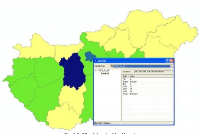
The query by location will answer the "what is here, what is in this point?" question. In general, the contents of the database remains unaffected, the GI system responses to your questions, fast, reliable and easily understandable way.

Fig. 1.2. What is here? – Identify tool

When you want information about a feature displayed in ArcMap, you can use the Identify tool on the Tools toolbar. The Identify tool allows you to see the attributes of your data and is an easy way to learn something about a location in a map. Clicking the Identify tool on a location inside a data frame will present the attributes of the data at that location. When identifying features with the Identify tool, the attributes are presented in a feature-by-feature, layer-by-layer manner in the Identify window.

Point-in-polygon

If you're looking for a point in a data layer that contains polygons, a "point-in-polygon" test must be carried out by the computer. Let us draw a line through the point, parallel with the coordinate axes. Define the intersections with the boundary of the polygon. Sort the points by their coordinates. If the point number is even, the point is within, if it is odd, than the point is outside of the polygon.

Fig. 1.3. „Point-in-polygon” test

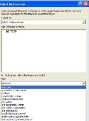
2.2. 1.2.2 Select by location

The Select By Location wizard (Fig. 1.4.) allows you select features based on their location relative to other features.

Fig. 1.4. In the query, you can choose from a long list of relationships.

Another example, if you want to know how many homes were affected by a recent flood (Fig. 1.5.). If you mapped the flood boundary, you could select all the homes that are within this area. Answering this type of question is known as a spatial query.

Fig. 1.5. Which settlements are in direct contact with rivers? Relationship between lines and polygons

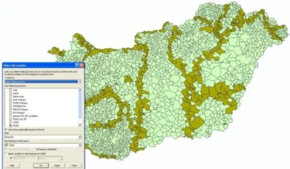
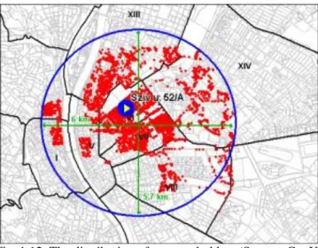
By combining queries, you can perform more complex searches. For example, suppose you want to find all the customers who live within a 30-kilometer radius of your store and who made a recent purchase so you can send them a promotional mailing.

Fig. 1.6. Select the polygons closer than 30 kilometers (intersect)

You can use a variety of selection methods to select the point, line, or polygon features in one layer that are near, or overlap the features in, the same or another layer.

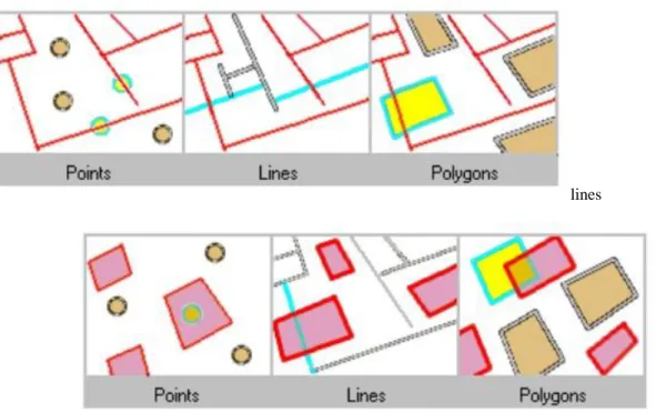
Intersect is the most generic operator. As its name implies, it will return any feature that geometrically shares a common part with the source feature (or features).

points

lines

Fig. 1.7. Explanation of the query using "Intersect" relation polygons

If you select by the „within” operator (instead of intersect), i.e. only those polygons, which in their entirety inside the window, the selected area would be reduced nearly by half. You need to decide what is really needed!

From the selected objects you may create a new layer (Create Layer From the Selected Features). Using the attribute table various reports could be created.

Fig. 1.8. Select polygons using intersect relation

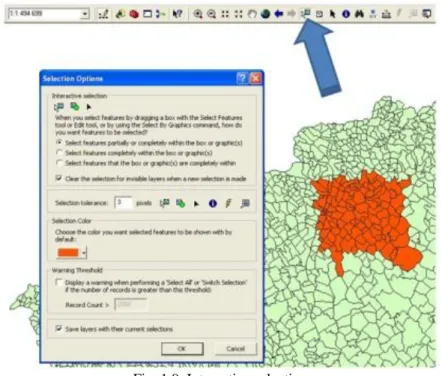
You can specify the selection criteria by the object properties (attribute data) for example: search for the polygons of which the land use is meadow or pasture, and the area of more than 5 ha). The selection can be done using a step-by-step approach when the selected dataset extended or narrowed by a new subset.

Fig. 1.9. Interactive selection

2.3. 1.2.3 Measurements

You can also perform measurements on the screen. You can measure the coordinates of each points, you can determine the distance between the selected points, you can query the area or perimeter of the polygons etc, all data can be measured like you were doing previously on the traditional graphic maps. The essential difference is that while the graphical map on paper distorted, the database (and thus the picture of the screen) will remain biased. The display resolution (in the illustration, Length = 342.34567890) is likely to deceive the inexperienced user. The accuracy of the coordinates, or other measured value is different, needs your investigations.

Fig. 1.10. Distance measurement

A further problem is the zoom, which must be consistent with the accuracy of the data in the database. If the scale is too small, the accuracy of the measurement is less than obtainable. If the scale is too large, the displayed numeric result can be misleading.

Let us not forget, therefore, that the accuracy of the result depends on the measurement accuracy on the screen and on the accuracy of the database.

2.4. 1.2.4 Visual interpretation

Sharing the resources between the human and the computer, one extreme case, when everything provided by the computer automatically (for example to produce a report ont he area of the polygons). On the other end, when the machine is used only for display, and the information produced by human interpretation. The man find solutions easier, in many cases, such as the computer (you will see an example in module 5, how to find errors in a digital elevation model by visual interpretation).

Fig. 1.11. Evaluation of the structure of real estates

The GIS software generally have quick navigation feature that eliminates the problems relating to the segmentation of traditional maps (map sheets), which allows you to jump more easily from the screen area to outsides. This resulted a seamless database from the user’s point of view.

The following figure illustrates the distribution of the account holders of a branch. You can detect that the account holders prefer the neighboring bank branches. But what does "neighboring" mean? The Euclidean distance is probably not the appropriate measure of the neighborhood! Another question: “Why do we find at the other side of the Danube so many account holders? These questions need more detailed analyses.

Fig. 1.12. The distribution of account holders (Source: GeoX) The following 3 figures give examples of the application of visual interpretation.

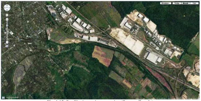
Fig. 1.13. Satellite image interpretation (Source: Google)

The vector database could be well complemented by the interpretation of satellite images and aerial photos.

Fig. 1.14. Visual analysis of the terrain surface

The color-band depiction of the terrain surface introduces a new dimension to topographic analysis, the flood hazard areas, or the zones with erosion danger can be selected easily. Digital elevation modeling will be discussed in Module 11.

Fig.1.15. The distribution of educational levels (Source: GeoX)

The figure paints an overview of educational image of the inhabitants of Budapest's. The dark green indicates of the lower, the dark red the higher level of education. I am sure that academicians also can live in Pest, but you can see the general trend. On the basis of the figure, what do you think about the price of real estates in Budapest?

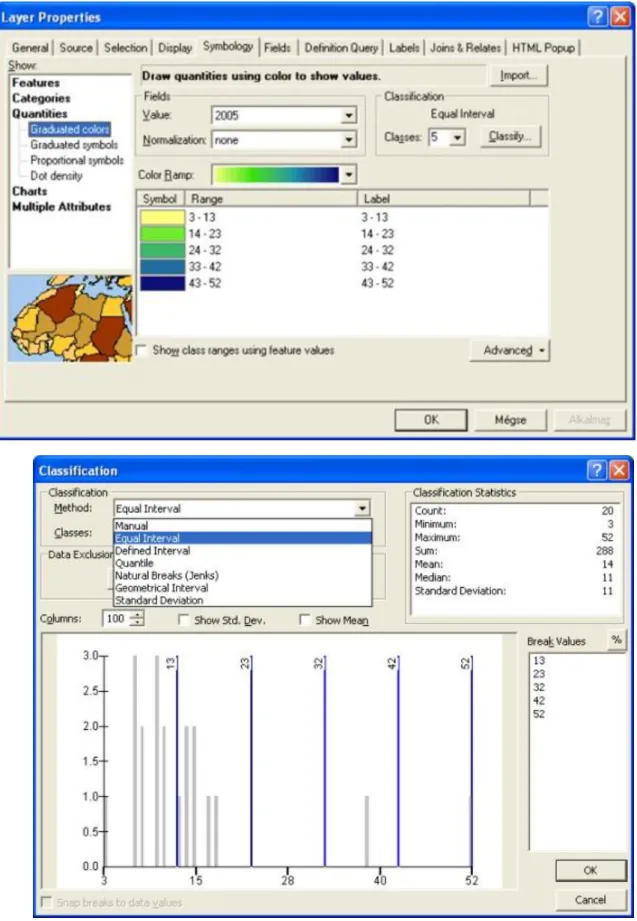
2.5. 1.2.5 Layer properties

The basic visualization tools can be found in the Layer Properties pop-up menu. You can see here the extent of the layer, the projection and coordinate system, the structure of attribute database etc.

The classification is supported by the basic statistical indicators:

• number of objects (count),

• minimal and maximal value of a selected attribute,

• sum of the values (sum),

• average (mean),

• median,

• standard deviation.

Fig. 1.16. The classification is supported by the basic statistical indicators and a frequency diagram The classification is attempting to create eye-catching, there are several ways to reach this aim:

• manual,

• equal interval,

Fig. 1.17. The distribution of full-time students of the Faculty of Geoinformatics equal interval – left side and quantile – right side (2005)

The zoom functions help to change quickly the scale of visualization, you can select the scale between sensible limits to enlarge or to decrease. However at the extremes generate a problem of reading the image or result misleading information. The minimum and maximum scale can be set in the Layer Properties menu.

3. 1.3 Select by attributes

Where is it? The „Select by Attributes” wizard helps to define query. After you open the wizard, the columns of the attribute table are displayed and its values are provided by request (Get unique values).

Fig. 1.18. Selection by attributes

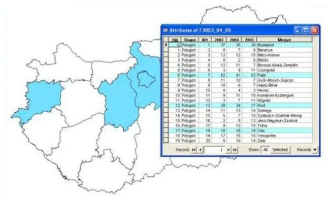
Fig 1.19. „From which counties were more than 15 students in 2005?"

The selection criteria can be specified by the object properties (descriptive data) For example: search for the polygons of which land use category is meadow or pasture, and the area is more than 5 ha). The selection criteria can be refined by Boolean parameters.

3.1. 1.3.1 Frequency diagram

A frequency diagram means of displaying raw data in a graphical form that is easier to interpret. The diagram used to record the number of times an event occurs.

We often need statistical data on the descriptive statements. The contents of the selected datasets, you can create various statistics (minimum, maximum, sum, mean, median, standard deviation etc.).

The diagram of the selected column of the attribute table describes the frequency of occurrence of specific values. The following illustration shows the frequency of occurrence of the land cover classes (code).

Fig. 1.20. Frequency diagram of a CORINE Land Cover 1:100 000 map sheet

4. 1.4 Topological search

In the databases with topological structure not only the „What is here?” and „Where is?” questions are easy, but the „Who/whereas neighbouring?” questions also could be answered in a natural way.

The topological data model from its nature provides a very effective search not only for the developers, but also the users.

The final section of the module extends the concept of transformation from geometrical operations to database transformations.

5.1. 1.5.1 Line weeding

Collecting data of linear objects often results very high point density. For example, the digitalization of contour lines often leads to too many points along with the contours, which can lead to errors in the height interpolation.

Therefore algorithms have been developed for line weeding.

Within ArcGIS two methods were developed to manage these problems (see next figure).

Fig. 1.24. Line weeding in ArcGIS (Source: ESRI)

The most often used algorithm developed by David Douglas and Thomas Peucker in 1973 .When weeding existing arcs in ArcGIS, the Douglas-Peucker algorithm is used to weed coordinates within each arc. The method is an algorithm for reducing the number of points in a curve that is approximated by a series of points.

The less-specific points could be deleted based (point remove) on the schema illustrated below.

Fig. 1.25. The concept of the Douglas – Peucker algorithm (Source: ESRI)

Fig. 1.26. The Douglas – Peucker algorithm for weeding contour lines „Simplify Line” command, 50 m simplification tolerance

The second algorithm (bend simplify) developed by Zeshen Wang. This uses a bend along the lines, examines the properties, and the points within the tolerance could be deleted.

5.2. 1.5.2 Merge

This operation combines input features from multiple input sources into a single, new, output feature class. The input data sources may be point, line, or polygon feature classes or tables.

The „merge” operation is required, particularly when after the digitalization of the map sheets you want to integrate the separate layers into a single, seemless database.

This looks like a simple task, but needs time-consuming, fine work, as long as the adjacent sections of the same objects can really merge and get rid of the boundary of the map sheets.

Fig. 1.27. Problems related to the adjacent contour lines at neighboring map sheets

Fig. 1.28. The concept of the merge operation (Source: ESRI)

5.3. 1.5.3 Split

The „split” operation clips portions of the input coverage into multiple coverages. The split coverage must have polygon topology. Each new output coverage contains only those portions of the input coverage features overlapped by the split coverage polygons.

The unique values in the Split Item are used to name the output coverages. Split Item values must be 13 characters or less. The number of output coverages is determined by the number of unique values in the Split Item.

Fig. 1.29. The concept of the „split” operation (Source: ESRI)

This operation is used, for example, to divide a national database into county databases. You can request, for example, provision from the national road database a county-based system. The feature attribute tables for the output coverage contain the same items as the Input Coverage attribute tables. The feature's internal number is used to transfer attribute information from the Input Coverage to each of the output coverages.

The following figure shows a portion of a land-use map which is divided into 1x1 km parts.

Fig. 1.30. Result of a „split” operation

5.4. 1.5.4 Dissolve

The „dissolve” operation creates a new coverage by merging adjacent polygons, lines, or regions that have the same value for a specified item.

Fig. 1.31. The concept of the „dissolve” operation (Source: ESRI)

Dissolve is used to create a simplified coverage from one that is more complex. Although the input coverage may contain information concerning many feature attributes, the output coverage contains information only about the dissolve item.

The merging of polygons with dissolve is the counterpart of intersecting polygons in overlays. Dissolve will remove the boundaries.

Dissolve maintains linear data belonging to different planar graphs in the same coverage. These may include arcs representing utility cables at different levels or a road passing over a stream. If there are arcs that appear to intersect, but do not, nodes will not be inserted at the apparent intersection. Coincident and colinear line segments are preserved; additional vertices may be inserted. Two colinear arcs, one representing a road that follows the second, a stream, are maintained colinear.

The soil database could be simplified using a „dissolve” command into a (watertight/not watertight) data layer to be created. The result is shown in the following figure.

Fig. 1.32. Dissolve deletes unnecessary borders (dissolve)

5.5. 1.5.5 Update and Append

The database maintenance is an essential daily task. To facilitate this, two solutions are presented here.

The „update” operation replaces the input coverage areas with the update coverage polygons using a cut and paste operation. The input coverage and the update coverage must have polygon topology.

Fig. 1.33. The concept of the „update” operation (Source: ESRI, available only in ArcInfo)

The operation appends multiple input datasets into an already existing target dataset. Input datasets can be point, line, or polygon feature classes; tables; rasters; or raster catalogs.

As an example of the work carried out, we can append on a daily basis newly measured data to the increasingly thriving central data base.

Fig. 1.34. The concept of the „append” operation (Source: ESRI)

5.6. 1.5.6 Raster-vector conversation

The raster-vector transformation is a common operation in geoinformatics, most of the time when remote- sensing data filled into a database, such as the following example shows. The example clearly shows that this action is associated with a significant loss of information. However, in view of the other side of the thing, the result can help you better understand and analyze the geographical area of interest.

Fig. 1.35. Raster-vector conversion – an example (Source: GISIG)

The aim of the CORINE (Coordination of Information on the Environment) project was to provide quantitative objective, reliable and comparable data in order to ensure the EU's land cover data. The data source was Landsat Thematic Mapper images made between 1990 and 1992. The vectorization was made manually by visual interpretation.

Fig. 1.36. CORINE land cover map, scale 1:100.000 (Source: FÖMI)

The automatic raster-vector transformation converts the (group of) pixels into vector objects (polygons, lines) by a computer algorithm. The following illustration shows how to derive the polygons boundary from the raster layer.

Fig. 1.37. Raster-vector conversion

The vector-raster conversion also an important, very often used operation. The definition of the parameters is supported by a wizard (see the following figure).

Fig. 1.38. The vector-raster conversion wizard (Source: ESRI)

Fig. 1.39. The result of a vector-raster conversion. Input: CORINE land cover map (see Fig. 1.36.) Output:

100x100 m raster

5.7. 1.5.7 Join

The attribute data records are linked through the ID (identification key) in the table, and the same ID in positional data. For example, the real estate ownership data are linked through the parcel ID to the cadastral map. If this table has more IDs, than more databases could be connected to the land-registry database (as illustrated int he following figure).

Fig. 1.40. Through the parcel ID (432) the ownership data are linked to the cadastral map

The “join table” operation joins a table view to a layer (or a table view to a table view) based on a common field. The records in the input layer or table view are matched to the record in the join table view based on the join field and the Input Field when the values are equal. The join is temporary, as is the layer, and will not persist from one session to the next unless the document is saved.

Fig. 1.41. The concept of „join table” operation (Add join)

6. 1.6 Summary

The aim of this module was, to give an overview of spatial data management and query operations, at the same time introduce the application. These operations appear in each GIS application, and support the GIS staff in operator level.

After mastering the material of the module, you are be able

• to determine the spatial database management functions,

• explain, what are the data management and query operations,

• discuss methods for handling a spatial database,

• give orientation in use of spatial queries.

Review questions

1. Describe the problems in the process, leading from data to the information!

2. Give an examples of the use of tolerances!

8. Give 3 examples for visual interpretation!

9. What are the main data provided by „Layer properties”, and what are possible options in the menu?

10. What are the main statistical indicators, you can use for the classification?

11. Explain the queries on the basis of the attribute data!

12. Describe the frequency diagram and the substance of the applicability.

13. Give algorithms for line weeding!

14. Describe the "merge", "split" and "dissolve" operations!

15. Describe how the "merge" and "split" command works!

16. Describe the "update" and "append" operations!

17. Explain the concept and use of „table join” operation!

Bibliography:

Márkus B.: Térinformatika, NyME GEO jegyzet, Székesfehérvár, 2009

Heywood, I. – Márkus B.: UNIGIS jegyzet, Székesfehérvár, 1999, http://webhelp.esri.com/

Detrekői Á. – Szabó Gy.: Térinformatika, Nemzeti Tankönyvkiadó, Budapest, 2002

Bernhardsen, T.: Geographic Information Systems – An Introduction, John Wiley & Sons, Inc., Toronto, 1999 NCGIA Core Curriculum: Bevezetés a térinformatikába (szerk. Márton M., Paksi J.), EFE FFFK,

Székesfehérvár, 1994