c World Scientific Publishing Company
COMPUTING ALL SPARSE KINETIC STRUCTURES FOR A LORENZ SYSTEM USING OPTIMIZATION
Zolt´an Andr´as Tuza1, G´abor Szederk´enyi1,2 *, Katalin M. Hangos2,3, Antonio A. Alonso4, Julio R. Banga4
1Faculty of Information Technology, P´eter P´azm´any Catholic University, Pr´ater u. 50/a Budapest, H-1083, Hungary
2Process Control Research Group, Systems and Control Laboratory, Computer and Automation Research Institute (MTA SZTAKI), Hungarian Academy of Sciences, P.O. Box 63
Budapest, H-1518, Hungary
3Department of Electrical Engineering and Information Systems, University of Pannonia, H-8200 Veszpr´em, Egyetem u. 10.
4(Bio)Process Engineering Group, IIM-CSIC, Spanish National Research Council, C/Eduardo Cabello, 6, 36208 Vigo, Spain
e-mails: tuza.zoltan@itk.ppke.hu, szeder@scl.sztaki.hu, hangos@scl.sztaki.hu, antonio@iim.csic.es, julio@iim.csic.es
Keywords: Lorenz system, kinetic systems, structural non-uniqueness, optimization
Received (to be inserted by publisher)
In this paper, all possible sparse chemical reaction network structures of a classical 3-dimensional Lorenz system are computed assuming a given chemical complex set. The original non-kinetic equations are transformed into kinetic form using two different approaches: firstly, using a state- dependent time-rescaling and secondly, by applying the theory of X-factorable systems. Using the notions of core reactions and core complexes, an effective optimization-based computation approach is proposed for the calculation of all structurally different sparse reaction graphs. The resulting structures are briefly analyzed and compared from a structural point of view.
1. Introduction
Kinetic systems (also called chemical reaction networks, or simply CRNs) are known to possess advanta- geous dynamical descriptive properties being able to produce all the important qualitative features like stable and unstable equilibria, multiple equilibria, bifurcation phenomena, oscillatory and even chaotic behaviour [Epstein & Pojman, 1998; ´Erdi & T´oth, 1989]. Many of these phenomena have actually been
∗corresponding author
1
observed in real chemical experiments where the practical constraints are much more severe than in the case of pure mathematical models [Noszticzius & B´odiss, 1980; Marlovitset al., 1995]. Thus, we can agree with the claim that the class of chemical reaction networks (CRNs) can be regarded as a possible “pro- totype of nonlinear science” [ ´Erdi & T´oth, 1989]. This fact may explain why kinetic systems have proved to be useful tools even in performing complex non-conventional computation tasks [De Lacy Costello &
Adamatzky, 2003; Adamatzkyet al., 2008, 2011]. Moreover, the simple algebraic structure of CRNs make these models attractive both for rigorous mathematical analysis and for efficient computational techniques [Horn & Jackson, 1972; Feinberg, 1987].
Kinetic systems can be used to describe pure chemical reactions or the complex dynamics of intra- cellular processes, metabolic or cell signalling pathways [Haag et al., 2005]. Thus, CRNs are suitable for modeling mechanisms both in industrial processes and in living environments. Based on these properties, it is clearly understandable why there has been an increasing interest towards chemical reaction networks among mathematicians and engineers recently [Sontag, 2001; Angeli, 2009; Chellaboina et al., 2009].
Necessary and sufficient conditions for a polynomial system to be kinetic were first given in [H´ars
& T´oth, 1981], where a constructive proof was given to build the so-called “canonic mechanism” for kinetic polynomial models. It has been known since at least the 1970’s that multiple different CRN struc- tures/parametrizations can generate exactly the same dynamics of the concentrations [Horn & Jackson, 1972; ´Erdi & T´oth, 1989]. This phenomenon is calledmacro-equivalenceordynamical equivalence. However, the exact geometric conditions of macro-equivalence were first studied relatively recently in [Craciun &
Pantea, 2008]. The first optimization-based numerical procedures for generating macro-equivalent struc- tures with prescribed (dynamically relevant) properties were published in [Szederk´enyi, 2010; Szederk´enyi et al., 2011b; Szederk´enyi & Hangos, 2011; Szederk´enyi et al., 2012].
It is known that the state-variables of kinetic systems are always nonnegative valued, since they com- monly describe the evolution of species concentrations in time. It is straightforward to show therefore that kinetic models mathematically belong to the family of nonnegative systems for which the nonnegative orthant is dynamically invariant [Haddad et al., 2010]. However, this important property is not neces- sarily an obstacle to the kinetic description of e.g. electric or mechanical systems: Firstly, in [Samardzija et al., 1989], the so-called X-factorable transformation is introduced that (together with an appropriate coordinates-translation) allows the kinetic representation of a wide class of dynamical systems. The second possibility is a coordinates-translation followed by a state-dependent time-rescaling, that is also suitable to transform originally non-kinetic models into kinetic form [Szederk´enyiet al., 2005; Hangos & Szederk´enyi, 2011]. Both of these approaches will be applied in this paper for the kinetic representation of the studied Lorenz system.
The kinetic realizations of certain chaotic systems have been studied previously in the literature.
In [Poland, 1993], a kinetic model of the Lorenz system was given by applying variable-translation and the assumption of slow reaction steps and constant concentrations of certain species. The nuclear spin generator (NSG) system is examined and transformed into chemical forms in [Xu & Li, 2002] using the methods published in [Samardzija et al., 1989] and [Poland, 1993], respectively. The first deterministic kinetic models of Chua’s circuit were presented in [Li & Xu, 2002] and [Xu & Li, 2003], while a stochastic simulator was described in [Li & Zhu, 2004].
The main purpose of this paper is to study the structural non-uniqueness of the kinetic realizations of dynamical systems using the example of the well-known Lorenz system. For this, an optimization- based approach is proposed for effectively computing all dynamically equivalent structures that contain the minimal number of reactions and thus provide a minimal parametrization of the system in terms of the reaction rate coefficients.
The structure of the paper is the following. In section 2, the notations and computational background for kinetic realizations of nolinear systems are given. The new contributions related to the applied method- ology and the computational results can be found in sections 3 and 4, respectively, while section 5 contains the conclusions of the reported work.
2. Background
This section summarizes the notions and methods corresponding to CRN representation and CRN structure computation. The description in this section is based on [Feinberg, 1979], [Szederk´enyi, 2010], [Szederk´enyi et al., 2011b] and [Szederk´enyi et al., 2011a].
2.1. Mathematical models of deterministic chemical reaction networks obeying the mass action law
We will use the commonly applied mathematical description of deterministic CRNs with mass action kinetics as it was given in e.g. [Feinberg, 1979]. In this formulation, a CRN is characterized by three sets:
(1) S ={X1, . . . , Xn} is the set ofspecies or chemical substances.
(2) C={C1, . . . , Cm} is the set ofcomplexes. Formally, the complexes are represented as linear combina- tions of the species, i.e.
Ci =
n
X
j=1
αijXj, i= 1, . . . , m, (1)
whereαij are nonnegative integers and are called thestoichiometric coefficients.
(3) R = {(Ci, Cj) | Ci, Cj ∈ C, i 6= j, andCi is transformed toCj in the CRN} is the set of reactions.
The relation (Ci, Cj) ∈ R will be denoted as Ci → Cj. Moreover, a nonnegative weight, the reaction rate coefficient denoted by kij is assigned to each reaction Ci → Cj. According to our convention, if the reaction Ci →Cj is not present in the CRN thenkij = 0.
It is important to remark that similarly to [Feinberg, 1987], the class of deterministic kinetic systems is considered here as a general nonlinear system class, and it is much wider than the family of chemically feasible kinetic systems. Therefore, we do not study the practical realizability of the obtained CRNs in this paper. We note that the existence of thermodynamically feasible CRN structures can be examined in the same optimization framework that we use in this paper by adding extra linear constraints (see, e.g.
[Szederk´enyi & Hangos, 2011]). Moreover, the realization computation techniques that are summarized in subsection 2.4, were successfully applied to biochemical models known from the literature in [Szederk´enyi et al., 2011a].
Given the setsS,CandR, a weighted directed graph (usually called the reaction graph)G= (V,E) can be constructed, where the setV contains the vertices that represent the complexes of the reaction network, i.e. V ={C1, C2, . . . , Cm}. The set E contains the directed edges representing the reactions between the complexes, i.e. (Ci, Cj) ∈ E if reaction Ci → Cj occurs in the CRN. Each directed edge (Ci, Cj) in the reaction graph is weighted by the rate coefficientkij. The undirected reaction graph obtained by replacing directed edges ofG with undirected ones will be denoted by|G|.
Now we briefly define the notions and properties of CRNs that will be used in the analysis of the computed structures. More details can be found in [Feinberg, 1987], while basic notions of directed graphs are discussed in e.g. [Bang-Jensen & Gutin, 2001]. First of all, linkage classes are maximal connected subgraphs (i.e. components) of G. That is, complexes Ci and Cj belong to the same linkage class if and only if there exists a path from Ci toCj in |G|. In the present paper, we do not treat isolated complexes without any outgoing or incoming edges (i.e. trivial connected components) as separate linkage classes, and we simply omit them from the CRN model (although we depict them in the figures for the sake of completeness). We call a reaction graph weakly reversible, if there exists a directed path from Ci to Cj
whenever there is a directed path fromCj toCi in the reaction graph.
To describe the time-evolution of species concentrations, we will use the following ODE form, which was applied e.g. in [Horn & Jackson, 1972]
˙
x=Y ·Ak·Ψ(x), (2)
wherex ∈Rn is the concentration vector of the species from S, and Y ∈ Rn×m is the called the complex composition matrix where the jth column encodes the composition of complex Cj as: Yi,j = αji. The
Ak ∈Rm×mmatrix stores the structure and parameters of the reaction graph. This is a column conservation matrix (also called the Kirchhoff matrix of the CRN) with nonpositive diagonal and nonnegative off diagonal entries is defined as follows:
[Ak]i,j =
−Pm
l=1,l6=ikil,if i=j
kji, ifi6=j. (3)
The last term in eq. (2), namely Ψ(x) = [ψ1(x) . . . ψm(x)]T, is a monomial-type vector mapping defined by
ψj(x) =
n
Y
i=1
xYii,j, j= 1, . . . , m. (4)
Clearly, because of eq. (4), we can uniquely define a CRN model with the matrix pair (Y, Ak).
To each reaction, we can associate a reaction vector denoted by eas
eij = [Y]·,j−[Y]·,i, (Ci, Cj)∈ R, (5) where [Y]·,idenotes theith column ofY. Therank of a network is the rank of the set of all reaction vectors in the CRN.
We have to discuss briefly the usage of the so-called zero complex in our models. The zero complex is formally represented by a zero column vector in Y, i.e. it is a special complex containing no species.
Similarly to [Feinberg, 1987], we use it to uniformly represent the environment, i.e. a CRN containing a (non-removable) zero complex is actually an open system. Therefore, the reactions of the type that are commonly written in the literature asS →X and X→P, whereS is a species of constant concentration and P is an unreactive product (the concentration of which is not included into the dynamic model), will be written as 0→X andX→0, respectively, where ‘0’ denotes the zero complex. Similarly, reactions like X+S →2X will be simply written asX →2X. It is emphasized that this is only a notational convention simplifying the description of CRNs. The resulting kinetic dynamics describing the concentrations in S are the same in both cases, and the two ways of representation can be easily transformed to each other, if necessary.
The structure of the reaction graph is directly connected with certain important dynamical properties of the CRN. The deficiency (a nonnegative integer number depending on the structure of the reaction graph and on complex composition but not on the particular values of reaction rate coefficients) is a good example for this [Feinberg, 1987]. The deficiency dof a CRN is given by the simple formula
d=m−l−s, (6)
wheremis the number of (non-isolated) complexes in the network,lis the number of linkage classes andsis the rank of the network. Roughly speaking, lower deficiencies (particularly 0 and 1) with certain structural properties like weak reversibility can guarantee an ‘ordered’ behaviour of kinetic dynamics without ‘exotic’
phenomena such as periodic solutions or chaos. Therefore, we do not expect that the deficiencies of the kinetic realizations of the studied Lorenz system will be low. Some examples of the direct consequences related to deficiency number such as the Deficiency One and Deficiency Zero Theorems can be found in [Feinberg, 1987].
2.2. Transformation of polynomial models into kinetic form
In this section, the background and the applied methods for transforming a general polynomial ODE system to kinetic form will be described.
2.2.1. Kinetic polynomial systems
Firstly, it is important to summarize when it is possible to assign a mass-action type CRN to a general polynomial dynamical system. In such a case, we call a dynamical system kinetic. The necessary and
sufficient condition for this that is easy to check, was first published in [H´ars & T´oth, 1981]. Consider an autonomous nonlinear system
˙
x=F(x), x∈Rn (7)
with polynomial right hand side. The system (7) is kinetic if and only if the coordinates functionsfi of F fulfill
fi(x) =−xig(x) +h(x), i= 1, . . . , n, (8) where g and h are polynomial functions with nonnegative coefficients. This means that all the negative monomial terms in the ith coordinate function of f must contain xi, i.e. negative cross-effects are not allowed in kinetic models.
In the constructive proof of the above condition in [H´ars & T´oth, 1981], a simple procedure is presented to build the so-called “canonical” CRN realization of a kinetic ODE. We briefly summarize this algorithm for convenience here, since we apply it later in Section 4 to compute the initial CRN corresponding to the Lorenz system transformed to kinetic form. Let the polynomial coordinates functions of the right hand side of a kinetic system (7) be given in the following form
fi(x) =
ri
X
j=1
mij n
Y
k=1
xbjk, i= 1, . . . , n, (9)
where ri is the number of monomial terms in fi. Let us denote the transpose of the ith standard basis vector in Rn as ei and let Bj = [bj1 . . . bjn]. Then, the steps necessary to construct the canonical CRN realization are the following.
Procedure 1 for computing the canonical CRN realization from [H´ars & T´oth, 1981]
For eachi= 1, . . . , nand for each j= 1, . . . , ri do:
(1) Qj: =Bj+ sign(mij)·ei
(2) Add the following reaction to the graph of the realization
n
X
k=1
bjkXk −→
n
X
k=1
qjkXk
with reaction rate coefficient|mij|, whereQj = [qj1 . . . qjn].
2.2.2. Transforming non-kinetic systems into kinetic form
In this section, we address the transformation of general polynomial ODEs not fulfilling the condition (8) into kinetic form using two different methods. First of all, we have to ensure that the trajectories of the system corresponding to the studied operating domain remain in the positive orthant. For this, the following simple translation of the state variables is used, if the positive orthant is not invariant for the original system’s dynamics:
¯
x=x+W, (10)
where the elements ofW = [w1 w2 . . . wn]T ∈Rnare sufficiently large that all trajectories of the translated system remain in the positive orthant if started from the studied initial conditions.
Now we describe the two distinct approaches, to transform our translated model into kinetic form.
State-dependent time-rescaling.Time-rescaling is a common operation in physical sciences. The par- ticular form of it depending on the positive state variables can be used e.g. for stability analysis of nonlinear systems (see [Gl´eria et al., 2001] and [Szederk´enyiet al., 2005]) or for motion control [Sz´adeczky-Kardoss
& Kiss, 2009]. In our case, the relationship between the original and transformed time-scales is defined by dt=
n
Y
i=1
xiχidτ, (11)
where tand τ are the time variables of the original and rescaled systems, respectively, and χi ∈ {0,1} for i= 1, . . . , n. It is important to stress that the positivity of the state variables implies that τ is a strictly monotonously increasing (and therefore invertible) function of t, and the phase-portraits of the original and rescaled models are identical. We will use the following notations for the derivative of x with respect tot andτ, respectively: ˙x= dxdt,x0 = dxdτ.
Clearly, the ODEs (7) corresponding to the new time-scale have the following form:
x0 =F(x)
n
Y
i=1
xiχi, (12)
from which it is easy to see thatχi can always be chosen such that the negative cross-effects are eliminated in the time-rescaled system.
X-factorable transformation. Another method for transforming a polynomial system into kinetic form was proposed in [Samardzijaet al., 1989]. A polynomial system of the form (7) is calledX-factorable if the right hand side of it can be factorized as
F(x) =D(x)G(x) (13)
where G ∈ Rn → Rn is a polynomial vector field and D(x) = diag{x1, x2, . . . , xn} ∈ Rn×n. It can be shown that the positive orthant for any X-factorable system is invariant for the dynamics [Haddad et al., 2010], and any X-factorable system is kinetic. Well-known examples of X-factorable systems are classical Lotka-Volterra models [Takeuchi, 1996].
Let us suppose that the solutions of (7) from a given set of initial conditions are strictly positive (possibly after a variable translation of the form (10)) but the model itself is not X-factorable. Then we assign the following transformed X-factorable model to the original one given by (7):
x˙˜=D(˜x)F(˜x), (14)
where again,D(˜x) = diag{˜x1,x˜2, . . . ,x˜n}. It is obvious that the phase-portraits of the two systems (7) and (14) are not identical in this case. However, under mild conditions, the system trajectories are ‘sufficiently similar’ in the interior of the positive orthant in the sense that the “distortion is weak or negligible for trajectories far from the boundary” of the positive orthant, while “a substantial compression of trajectories occurs close to the boundary” [Samardzijaet al., 1989]. Moreover, the behaviour of (14) around the strictly positive equilibrium points is essentially dynamically equivalent to that of (7) [Samardzijaet al., 1989].
2.3. Dynamical equivalence of mass-action networks
Now we formally define the dynamical equivalence (or macro-equivalence) of reaction networks that has already been mentioned in the Introduction. Let us define two CRNs with the following matrix pairs (Y(1), A(1)k ) and (Y(2), A(2)k ). We call these CRNs dynamically equivalent, if
Y(1)A(1)k ψ(1)(x) =Y(2)A(2)k ψ(2)(x), ∀x∈R¯n+, (15) where for i = 1,2, Y(i) ∈ Rn×mi have nonnegative integer entries, A(i)k are valid Kirchhoff matrices, ¯Rn+
denotes the closed nonnegative orthant and ψj(i)(x) =
n
Y
k=1
x[Y
(i)]k,j
k , i= 1,2, j = 1, . . . , mi. (16) We will assume that the set of complexes are fixed and known before the computations, therefore (15) can be rewritten as
Y ·A(1)k =Y ·A(2)k =:M (17)
withM being the invariant matrix containing the coefficients of the monomials in the kinetic polynomial ODEs.
Clearly, if A(1)k and A(2)k give dynamically equivalent realizations with fixed Y, then A(3)k = A
(1) k +A(2)k
2
also gives a valid dynamically equivalent realization with Y. Therefore, a kinetic system with different dynamically equivalent realizations has infinitely many dynamically equivalent realizations. Thus, we can apply computational methods to calculate those realizations that fullfil predefined properties such as density or sparsity, weak reversibility, etc. The detailed description of these methods can be found in [Szederk´enyi, 2010; Szederk´enyi et al., 2012, 2011b,a].
2.4. Known optimization methods for computing certain CRN realizations
In this subsection, we briefly recall the computation framework first described in [Szederk´enyi, 2010] and some related results for convenience. For a fixed complex composition matrixY,sparse realizationscontain the minimum number of nonzero off-diagonal elements (i.e. reactions) in theAkmatrix. On the other hand dense realizations contain the maximal number of nonzero off-diagonal elements inAk. These calculations can be formulated as mixed integer linear programing (MILP) problems, where we assume that we have a canonical CRN and its parameters are known. Solving the MILP optimization, we want to find other valid Ak Kirchhoff matrices that fulfill the given requirements.
The mass-action dynamics can be expressed as equality and inequality constraints as
Y ·Ak=M (18)
m
X
i=1
[Ak]ij = 0, j= 1, . . . , m (19)
[Ak]ij ≥0 i, j= 1, . . . , m i6=j (20)
[Ak]ii≤0, i= 1, . . . , m (21)
where the elements ofAk are the decision variables. We also put lower and upper bound constraints on the decision variables to make the optimization problem computationally tractable and to avoid unbounded feasible solutions.
0≤[Ak]ij ≤lij, i, j = 1, . . . , m, i6=j (22)
lii≤[Ak]ii ≤0, i= 1, . . . , m (23)
Using these constraints we can find suchAk matrices where the number of nonzero off-diagonal elements are minimal or maximal. To achieve this, we introduce logical variables denoted by δ and construct the following compound statements.
δij = 1↔[Ak]ij > , i, j= 1, . . . , m, i6=j (24) where ‘↔’ encodes theif and only if logical statement, is an arbitrary small threshold variable (below the value of, we treat the corresponding reaction rate as zero in the reaction graph). The inequalities in (22) and (24) can be combined into the following form [Raman & Grossmann, 1994]
0≤ [Ak]ij−δij i, j= 1, . . . , m, i6=j (25) 0≤ −[Ak]ij+lijδij ≤0, i, j= 1, . . . , m, i6=j (26) The function summing the nonzero reaction rate coefficients is:
h(δ) =
m
X
i,j=1i6=j
δij. (27)
By maximizing or minimizingh(δ), we are able to compute realizations with maximal or minimal number of reactions, i.e. the dense or sparse realizations of a canonical CRN.
As section 4 will illustrate, sparse realizations are structurally non-unique, meanwhile the structure of the dense realization with a given complex set is unique and contains every possible dynamically equivalent structure as a proper subgraph, i.e. it is a kind of superstructure [Szederk´enyi et al., 2011b].
The dynamically equivalent realizations share some common structural elements that are essential for the equivalence. The so-called core complexes and core reactions belong to these important elements.
Core complexes are those vertices of the reaction graph that are present as reactants or products in any dynamically equivalent realizations of a given CRN. It is easy to observe that a complex is non-reacting (or isolated) in a CRN realization, if both the corresponding row and colum ofAk contains only zeros (i.e.
there are no incoming or outgoing directed edges to/from that complex in the reaction graph). Based on this, we can formulate a simple test to find core complexes. The complexCk is a core complex if and only if the constraint
m
X
i= 1 i6=k
[Ab]ki+
m
X
j= 1 j6=k
[Ab]jk = 0 (28)
together with (18)-(21) is infeasible. Since no integer variable is involved in this constraint, core complexes can be found with linear programming (LP).
Similarly to core complexes, core reactions are present (possibly with different rate coefficients) in any dynamically equivalent realization of a CRN [Szederk´enyiet al., 2011a]. Whether a reaction belongs to the set of core reactions or not, can be tested with simple linear programming, too. Therefore, Ci → Cj is a core reaction if and only if (18)-(21) with
[Ak]ji = 0 (29)
yields an infeasible LP problem. From now on, we will denote the number of reactions in the dense and sparse realizations withRdandRs, respectively, and the number of core reactions and core complexes with Rcand Nc, respectively.
We remark that it is straightforward to extend the notions of dense and sparse realizations together with core reactions and core complexes to the constrained case, when some of the mathematically possible reactions are a’priori excluded from the reaction network by setting the appropriate elements ofAkto zero.
The notations for this are the following. The simple constraint set denoted by K used for the exclusion of selected reactions from the CRN is given by:
K ={[Ak]i1,j1 = 0, . . . , [Ak]is,js = 0}, (30) wheresis the number of individual constraints, andik 6=jkfork= 1, . . . , s. Then, a dynamically equivalent K-constrained realization of a CRN (Y, Ak) is a reaction network (Y, A0k) such thatY ·Ak=Y·A0kand the prescribed constraintsK in the form of eq. (30) are fulfilled forA0k. A dynamically equivalentK-constrained dense realization of a chemical reaction network (Y, Ak) is a K-constrained realization that contains the maximal number of nonzero elements inA0k. Similarly, aK-constrained sparse realizationis aK-constrained realization with the minimal number of nonzeros in A0k. Naturally, a dynamically equivalent constrained realization may not exist for certain constraint sets, therefore the existence of such realizations must be checked through the feasibility of the corresponding optimization problem.
It is also true in this case that for a fixed complex and constraint set, the dense realization gives a maximal superstructure of all possible realizations [Szederk´enyi et al., 2011a]. Moreover, it is important to note here that the computation of constrained dense realizations can be traced back to a series of pure LP steps [Szederk´enyi et al., 2011a] and therefore it can be performed in polynomial time, while the computation of a sparse realization without any prior knowledge about Rd and Rs still requires integer variables and MILP computations.
3. Computation of all possible sparse structures
In this section, we present a computational approach to calculate all possible dynamically equivalent sparse CRN structures. Firstly, we describe the main ideas behind the applied computation method. We exploit the above described fact that the structure of the dense realization of a CRN is unique, and it contains the structures of all possible dynamically equivalent realizations as sub-graphs. The first step is the computation of an arbitrary sparse and dense realization of the studied kinetic system to determine Rs and Rd. Then,
we extract all possible sparse structures by ‘pulling down’ the dense one. For this, it is clear that we have to remove as many reactions from the dense realization (if possible) as the difference between the number of reactions in the dense and sparse realizations, i.e. Rd−Rs. By ‘removing’ a reaction from a CRN, we mean that the corresponding reaction rate coefficient in Ak is made zero while maintaining dynamical equivalence with the initial kinetic system. Using only the fact that core reactions are not removable from any realization, the maximal theoretical number of possibilities to be checked is
Nmax=
Rd−Rc Rd−Rs
= (Rd−Rc)!
(Rd−Rs)!(Rs−Rc)!. (31)
This means that in the worst case, we have to checkNmax possibilities for dynamical equivalence, where each checking requires the solution of an LP problem with constraints (18)-(23) and (30). As we will see later in the case of the Lorenz system,Nmaxcan be so large even in the case of a small network, that it might be computationally infeasible to check all possibilities individually. To ease the computational burden, we identify the set of reaction pairs (denoted byR2e ⊂ R × R) which are non-core reactions, but if any reaction pair from R2e is not present in a given reaction graph, then the corresponding dynamically equivalent realization cannot be sparse. In other words, the exclusion of any reaction pair from R2e always implies the inclusion of more than 2 other reactions in the reaction graph, and this clearly violates the sparsity constraint. Knowing this information, we can omit from the systematic search those realizations that do not contain any pair fromR2e, and this can drastically reduce the overall computation time. The computational background for determiningR2e is simple: any pair of distinct reactions Rp = (Ci →Cj, Ck→Cl) belongs to R2e if and only if the constrained sparse realization not containing the elements of Rp contains more reactions than the original unconstrained sparse realization. This means that determining Rpe requires Rd−Rc
2
MILP optimizations steps.
Let us introduce the following additional notations. LetP(S) denote the power set of an arbitrary set S, and let |S|be the cardinality of S. Let R(Y, Ak) denote the set of reactions of a CRN with complex composition matrix Y and Kirchhoff matrix Ak. Furthermore, let Pk(S) denote the elements (sets) of P(S) containingk elements, i.e. Pk(S) ={A∈ P(S) | |A|=k}. Now we can summarize the computation steps for determining all sparse realization structures more formally as follows (the sparse realizations with different structures are collected into the set calledSparse structs).
1. LetSparse structs:=∅.
2. Determine the canonical realization (Y, Ack) of the studied kinetic system usingProcedure 1.
3. Compute a dense realization (Y, Adk) of (Y, Ack). LetRd:=|R(Y, Adk)|.
4. Compute a sparse realization (Y, Ask) of (Y, Ack). Let Rs:=|R(Y, Ask)|.
5. Identify the set of core reactionsRcof (Y, Ack). Let Rc:=|Rc|.
6. LetR2e :=∅.
7. For each pair of distinct reactions {Ci→Cj, Ck →Cl} inR(Y, Adk)\ Rc do:
7.1. LetK1:={[Ak]j,i= 0, [Ak]l,k= 0}.
7.2. Compute aK1-constrained sparse realization (Y, AKk1) of (Y, Adk).
7.3. If (Y, AKk1) exists and |R(Y, AKk1)|> Ns then let R2e :=R2e∪(Ci→Cj, Ck →Cl).
8. Letz:=Rd−Rs.
9. LetRz :=Pz(R(Y, Adk)\ Rc).
10. For eachRi={Ci1 →Cj1, . . . , Ciz →Cjz} ∈ Rz do:
10.1. IfRi does not contain any reaction pair from R2e then do:
10.1.1. Let K2 :={[Ak]j1,i1 = 0, . . . ,[Ak]jz,iz = 0}.
10.1.2. Compute aK2-constrained realization (Y, AKk2) of (Y, Adk).
10.1.3. If (Y, AKk2) exists, then letSparse structs:=Sparse structs∪ (Y, AKk2).
For the generation of Rz, we applied the fast algorithm described in section 7.2.1.3 of [Knuth, 2008].
We emphasize again that integer variables are required only for steps 4 and 7.2 of the above algorithm, and all other realizations can be computed by standard linear programming. We remark that after the
initialization steps 1-6, the necessary time for the subsequent computations can be pre-estimated quite precisely, knowing the average time required for a MILP or LP realization computation step.
4. Results: sparse kinetic realizations of the Lorenz system
The starting point is the classical set of equations corresponding to the Lorenz system:
˙
x1 =σ(x2−x1)
˙
x2 =ρx1−x2−x1x3 (32)
˙
x3 =x1x2−βx3
with parameter values σ = 10, ρ = 28, β = 8/3 that are known to lead to chaotic behaviour. It is also known that the nonnegative orthant is not invariant for the original dynamics (32), therefore firstly a coordinates-translation was applied with W =
24,25,26
. The principles for selecting the elements of W were the following. Firstly, they should be as small as possible while allowing the shift of the studied operating domain to the strictly positive orthant. Secondly, they should be different in order to avoid any monomial cancellations later in the kinetic models. The translated model reads:
˙¯
x1 =σx¯2−σx¯1+σ(w1−w2)
˙¯
x2 = (ρ+w3)¯x1−x¯2+w1x¯3−x¯1x¯3−ρw1+w2−w1w3 (33)
˙¯
x3 = ¯x1x¯2−w2x¯1−w1x¯2+w1w2−βx¯3+βw3 4.1. State-dependent time-rescaling
It is easy to see that the set of ODEs (33) is generally not kinetic. Therefore, we apply the most general time-scaling that contains all 3 state variables, namely dt= ¯x1x¯2x¯3dτ. The rescaled kinetic equations are written as
¯
x01=σx¯1x¯22x¯3−σx¯21x¯2x¯3+σ(w1−w2)¯x1x¯2x¯3
¯
x02= (ρ+c3)¯x21x¯2x¯3+ (w2−w1ρ−w1w3)¯x1x¯2x¯3−x¯1x¯22x¯3−x¯21x¯2x¯23+w1x¯1x¯2x¯23 (34)
¯
x03= ¯x21x¯22x¯3−w2x¯21x¯2x¯3−w1x¯1x¯22x¯3+ (w1w2+βw3)¯x1x¯2x¯3−βx¯1x¯2x¯23
The simulated system trajectories of (34) are shown in Figure 1(a). Let us denote the species corresponding to the concentrations ¯x1,x¯2 and ¯x3 by X1, X2 and X3, respectively. Then,Procedure 1for building the canonical structure (described in Subsection 2.2.1) generates the following complex set for the canonical realization of (34)
C1 =X1+X2+X3, C2 =X2+X3, C3 = 2X1+X2+X3, C4 =X1+ 2X2+X3,
C5 = 2X1+ 2X2+X3, C6=X1+X3, C7=X1+X2+ 2X3, C8=X1+ 2X2+ 2X3, (35) C9 = 2X1+X2+ 2X3, C10= 2X1+ 2X3, C11= 2X1+X2, C12=X1+ 2X2, C13= 2X1+ 2X2+ 2X3
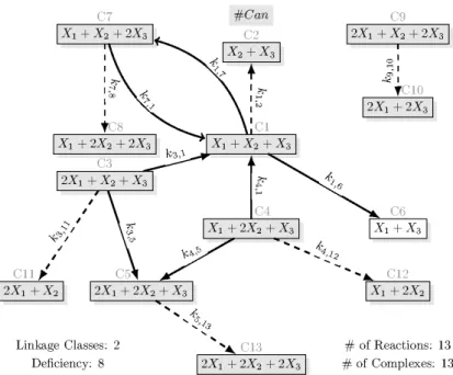
The canonical reaction network corresponding to (34) is shown in Figure 2, which shows the reaction rate coefficients on the directed edges. The core reactions and core complexes are indicated by dashed arrows and grey rectangles, respectively in all figures showing CRN structures. The 6 core reactions of the system are the following:
C1 →C2, C3→C11, C4→C12, C5 →C13, C7 →C8, C9→C10.
Moreover, all complexes in (35) are core complexes with the exception of C6 =X1+X3. We remark that the canonical realization can be computed symbolically, but the optimization techniques for computing the forthcoming dense and sparse realizations are numerical, and they use the previously described model parameter values.
To compute all possible sparse structures of this CRN, we need further information such as the possible minimal and maximal number of reactions and also the set of core reactions. Using the computation
methods described in section 2, we can easily obtain these data. The values of the realization parameters in the case of the time-rescaled model are the following: Rd = 51, Rs = 13, Rc = 6, and Nc = 11. The value ofNmax(i.e. the maximal number of required LP steps to check all possibilities) is 45.379.620 in this case which would require about 630 hours of computation time on the desktop PC that we used, assuming approximately 0.05 s for one LP step.
In the case of the time-rescaled model (34),Pe2 was found to be the following:
Pe2 ={(C3 →C5, C3→C13),(C4 →C5, C4 →C13),(C1→C6, C1 →C10),(C1 →C6, C1→C11)} (36) Using Pe2, the search space was reduced to 442.454 possibilities, that is a huge reduction compared to the initial more than 45 million. After checking the candidate realizations with the method described in section 3, we found that 5376 different structures are valid dynamically equivalent sparse realizations. Out of these, 504 are such that they contain only the 11 core complexes.
4.2. X-factorable transformation
Besides the state-dependent time-scaling, we also investigated the 3-dimensional Lorenz system with the X-factorable transformation. Firstly, we again performed a coordinates shift on model (32) and then applied the X-factorable transformation. The resulting equations are
˙˜
x1 =σx˜1x˜2−σx˜21−σ(w1−w2)˜x1
x˙˜2 = (w3+ρ)˜x1x˜2−x˜22+w1x˜2x˜3−x˜1x˜2x˜3+ (w2−w1ρ−c1c3)˜x2 (37) x˙˜3 = ˜x1x˜2x˜3−w1x˜2x˜3−w2x˜1x˜3+ (w1w2+βw3)˜x3−βx˜23,
whereW =
100,101,1
, which is basically taken from [Samardzija et al., 1989], but w2 is modified from 100 to 101 to avoid cancellation of the last monomial in the first equation.
Again, usingProcedure 1, the complexes of the canonical realization are given as C1 =X1, C2= 0, C3= 2X1, C4=X1+X2, C5= 2X1+X2, C6 =X2,
C7 = 2X2, C8 =X1+ 2X2, C9 =X2+X3, C10= 2X2+X3, C11=X1+X2+X3, (38) C12=X1+X3, C13=X3, C14= 2X3, C15=X1+X2+ 2X3,
where the speciesX1,X2 andX3 correspond to the state variables ˜x1, ˜x2 and ˜x3 of (37), respectively.
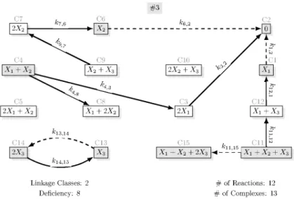
The reaction graph of the canonical realization is shown in Figure 6. The list of core reactions is
C1 →C2, C6→C2, C11→C15, C13→C14, (39) while the core complexes are C1,C2, C4,C6, C13, C14, C15. The characteristic parameter values for this network areRs= 12, Rd= 44,Rc= 4. andNc= 8.
The value of Nmax is 76.904.685 that would require about 1068 hours of computation time to check each possible combination. ForPe we obtained:
Pe2 ={(C3→C1, C3 →C2),(C12→C1, C12→C3),(C7 →C2, C7 →C6),(C14→C2, C14→C13), (40) (C4→C3, C4 →C5),(C4 →C5, C4 →C8),(C4 →C7, C4→C8),(C9→C7, C9 →C10)}.
After checking the possible sparse graph structures, we found that only 2864 do not contain any pair from Pe2, which is only 0.0037% of the original nearly 77 million possibilities. It was computationally easy to check these 2864 candidates, among which we found only 48 valid dynamically equivalent sparse realization structures. In this case, there was no such realization that only contained the core complexes.
Due to the large number of dynamically equivalent structures, the reaction graphs for all sparse realizations from both methods are provided in an electronic supplement downloadable from http://daedalus.scl.sztaki.hu/PCRG/works/Suppl2012 001.pdf. Therefore, only a few character- istic examples are included in the main text of the paper. The core reactions and core complexes are indicated by dashed arrows and grey boxes, respectively in the figures. The numbers of the complexes are written above the boxes containing the complexes. The unique identification numbers (serial numbers) of the sparse structures are indicated at the top of the figures. The isolated (unconnected) complexes are
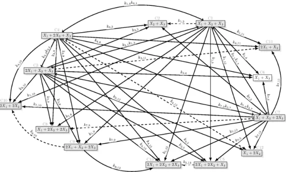
omitted from the models but they are drawn in the figures for easier comparison. The superstructures (i.e.
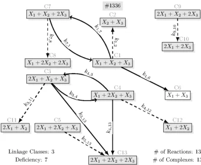
the dense realizations) are shown in Figs 5 and 8, respectively. Fig. 3 shows a sparse realization of (34) with the maximal number of linkage classes (three), while a sparse realization of (34) containing only the 11 core complexes can be seen in Fig. 4. From the 48 sparse realizations of (37), Fig. 7 shows one with the minimal number of complexes (13).
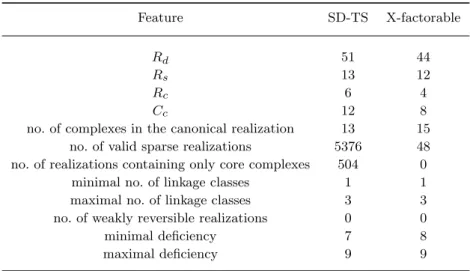
The brief comparison of the time-rescaling and X-factorable transformation cases can be found in Table 6. As the table shows, we haven’t found any weakly reversible realizations among the sparse ones. This means that there are no sparse complex balanced realizations with the given complex sets, since it is known that complex balancing implies weak reversibility [Horn, 1972]. Moreover, the deficiencies of all obtained sparse CRNs are high (between 7 and 9) that is related to the dynamical complexity of the network.
5. Conclusions
Dynamically equivalent sparse kinetic realizations of a classical Lorenz system were computed in this paper. The optimization-based computational framework proposed originally in [Szederk´enyi, 2010] was successfully used to solve this task. The set of complexes for the realizations was generated using the procedure published in [H´ars & T´oth, 1981]. The original model was transformed to kinetic form using two different approaches known from literature: the state-dependent time-rescaling that completely preserves the structure of the phase-space, and the X-factorable transformation. Firstly, the essential components (i.e. the core reactions and core complexes) of the networks have been determined. The studied realization computation problem is clearly of combinatorial nature, therefore an effective reduction of the search space was proposed using core complexes and the advantageous properties of dense realizations. All different sparse structures are listed in an electronic supplement. The large number of valid solutions clearly illustrate the possible structural non-uniqueness of chemical reaction networks. To the best of the authors’ knowledge, it has been the first attempt to enumerate all dynamically equivalent structures of a kinetic dynamical system with a given property.
6. Acknowledgements
This research has been partially supported by the Hungarian National Research Fund through grant no.
OTKA NF 104706. The support of projects T ´AMOP-4.2.1.B-11/2/KMR-2011-0002 and T ´AMOP-4.2.2/B- 10/1-2010-0014 as well as the support of the Marginal Research Association of Budapest are also gratefully acknowledged. G. Szederk´enyi and Z. A. Tuza thank Prof. Tam´as Roska for the stimulating discussions.
References
Adamatzky, A., De Lacy Costello, B. & Bull, L. [2011] “On polymorphic logical gates in subexcitable chemical medium,”International Journal of Bifurcation and Chaos 21, 1977–1986.
Adamatzky, A., De Lacy Costello, B. & Shirakawa, T. [2008] “Universal computation with limited resources:
Belousov-Zhabotinsky and physarum computers,”International Journal of Bifurcation and Chaos18, 2373–2389.
Angeli, D. [2009] “A tutorial on chemical network dynamics,” European Journal of Control 15, 398–406.
Bang-Jensen, J. & Gutin, G. [2001] Digraphs: Theory, Algorithms and Applications (Springer).
Chellaboina, V., Bhat, S. P., Haddad, W. M. & Bernstein, D. S. [2009] “Modeling and analysis of mass- action kinetics – nonnegativity, realizability, reducibility, and semistability,” IEEE Control Systems Magazine 29, 60–78.
Craciun, G. & Pantea, C. [2008] “Identifiability of chemical reaction networks,” Journal of Mathematical Chemistry 44, 244–259.
De Lacy Costello, B. & Adamatzky, A. [2003] “On multitasking in parallel chemical processors: Experi- mental findings,” International Journal of Bifurcation and Chaos 13, 521–533.
Epstein, I. R. & Pojman, J. A. [1998] An Introduction to Nonlinear Chemical Dynamics: Oscillations, Waves,Patterns and Chaos (Topics in Physical Chemistry) (Oxford University Press).
Feinberg, M. [1979] Lectures on chemical reaction networks (Notes of lectures given at the Mathematics Research Center, University of Wisconsin).
Feinberg, M. [1987] “Chemical reaction network structure and the stability of complex isothermal reactors - I. The deficiency zero and deficiency one theorems,”Chemical Engineering Science 42 (10), 2229–
2268.
Gl´eria, I. M., Figueiredo, A. & Filho, T. M. R. [2001] “Stability properties of a general class of nonlinear dynamical systems,”Journal of Physics A - Mathematical and General 34, 3561–3575.
Haag, J., Wouver, A. & Bogaerts, P. [2005] “Dynamic modeling of complex biological systems: a link between metabolic and macroscopic description,”Mathematical Biosciences 193, 25–49.
Haddad, W. M., Chellaboina, V. & Hui, Q. [2010] Nonnegative and Compartmental Dynamical Systems (Princeton University Press).
Hangos, K. M. & Szederk´enyi, G. [2011] “Mass action realizations of reaction kinetic system models on various time scales,”Journal of Physics: Conference Series (5th International Workshop on Multi-Rate Processes and Hysteresis (MURPHYS 2010))268, 012009, doi:10.1088/1742-6596/268/1/012009.
Horn, F. [1972] “Necessary and sufficient conditions for complex balancing in chemical kinetics,” Archive for Rational Mechanics and Analysis 49, 172–186.
Horn, F. & Jackson, R. [1972] “General mass action kinetics,”Archive for Rational Mechanics and Analysis 47, 81–116.
H´ars, V. & T´oth, J. [1981] “On the inverse problem of reaction kinetics,”Qualitative Theory of Differential Equations, eds. Farkas, M. & Hatvani, L. (North-Holland, Amsterdam), pp. 363–379.
Knuth, D. E. [2008] The Art of Computer Programming, Volume 4A, Combinatorial Algorithms, Part 1 (Addison-Wesley Professional).
Li, Q. & Xu, W. [2002] “A chemical model for Chua’s equation,”International Journal of Bifurcation and Chaos 12, 877–882.
Li, Q. & Zhu, R. [2004] “Stochastic simulation of chemical chua system,” International Journal of Bifur- cation and Chaos 14, 1053–1057.
Marlovits, G., Wittmann, M., Noszticzius, Z. & G´asp´ar, V. [1995] “A new chemical oscillator in a novel open reactor - the CLO2-I-2-Acetone system in a membrane fed stirred tank reactors,” Journal of Physical Chemistry 99, 5359–5364.
Noszticzius, Z. & B´odiss, J. [1980] “Contribution to the chemistry of the Belousov-Zhabotinskii (BZ) type reactions,”Berichte der Bunsen-Gesellschaft - Physical Chemistry Chemical Physics 84, 366–369.
Poland, D. [1993] “Cooperative catalysis and chemical chaos: a chemical model for the lorenz equations,”
Physica D: Nonlinear Phenomena 65, 86–99.
Raman, R. & Grossmann, I. [1994] “Modelling and computational techniques for logic based integer pro- gramming,”Computers and Chemical Engineering 18, 563–578.
Samardzija, N., Greller, L. D. & Wassermann, E. [1989] “Nonlinear chemical kinetic schemes derived from mechanical and electrical dynamical systems,”Journal of Chemical Physics 90 (4), 2296–2304.
Sontag, E. [2001] “Structure and stability of certain chemical networks and applications to the kinetic proofreading model of T-cell receptor signal transduction,”IEEE Transactions on Automatic Control 46, 1028–1047.
Szederk´enyi, G. [2010] “Computing sparse and dense realizations of reaction kinetic systems,” Journal of Mathematical Chemistry 47, 551–568, doi:10.1007/s10910-009-9525-5, URL http://www.springerlink.
com.
Szederk´enyi, G., Banga, J. R. & Alonso, A. A. [2011a] “Inference of complex biological networks:
distinguishability issues and optimization-based solutions,” BMC Systems Biology 5, 177, doi:
10.1186/1752-0509-5-177.
Szederk´enyi, G., Hangos, K. & Magyar, A. [2005] “On the time-reparametrization of quasi-polynomial systems,”Physics Letters A 334, 288–294, doi:10.1016/j.physleta.2004.11.026.
Szederk´enyi, G. & Hangos, K. M. [2011] “Finding complex balanced and detailed balanced realiza- tions of chemical reaction networks,” Journal of Mathematical Chemistry 49, 1163–1179, doi:
10.1007/s10910-011-9804-9.
Szederk´enyi, G., Hangos, K. M. & P´eni, T. [2011b] “Maximal and minimal realizations of reaction kinetic
systems: computation and properties,”MATCH Commun. Math. Comput. Chem. 65, 309–332.
Szederk´enyi, G., Hangos, K. M. & Tuza, Z. [2012] “Finding weakly reversible realizations of chemical reaction networks using optimization,”MATCH Commun. Math. Comput. Chem.67, 193–212, URL http://arxiv.org/abs/1103.4741.
Sz´adeczky-Kardoss, E. & Kiss, B. [2009] “On-line trajectory time-scaling to reduce tracking error,”Intel- ligent Engineering Systems and Computational Cybernetics (Springer), pp. 3–14.
Takeuchi, Y. [1996]Global Dynamical Properties of Lotka-Volterra Systems (World Scientific, Singapore).
Xu, W. & Li, Q. [2002] “Chemical chaotic schemes derived from NSG system,”Chaos, Solitons and Fractals 15, 663–671.
Xu, W. & Li, Q. [2003] “Another chemical chaotic attractor for chua’s equation,”International Journal of Bifurcation and Chaos 13, 2715–2718.
Erdi, P. & T´´ oth, J. [1989]Mathematical Models of Chemical Reactions. Theory and Applications of Deter- ministic and Stochastic Models (Manchester University Press, Princeton University Press, Manchester, Princeton).
Figures
Fig. 1. (a) Phase-plane plot of the kinetic Lorenz system obtained via time-rescaling (left), (b) Phase-plane plot of the Kinetic Lorenz system obtained using the X-factorable transformation (right).
Fig. 2. Canonical realization of the Lorenz system with state-dependent time-scaling. In this case, the canonical realization is also a sparse one. The parameters are:k3,1=σ,k4,1= 1,k7,1=β,k1,2=σ,k3,5=ρ+w3,k4,5=σ,k1,6=|w2−w1ρ−w1w3|, k1,7=w1w2+βw3,k7,8=w1,k9,10=σ,k3,11=w2,k4,12=w1,k5,13=σ.
Fig. 3. Sparse realization of the model (34) with 3 linkage classes. The reaction rate coefficients are:k7,1= 2.6667,k1,2= 10, k4,3= 1,k3,4= 10,k1,6= 1271,k1,7= 699.33,k7,8= 24,k9,10= 1,k3,11= 69,k4,12= 33,k3,13= 44,k4,13= 9,k5,13= 1.
Fig. 4. Sparse realization of the model (34) that contains only the core complexes. The reaction rate coefficients are:k1,2= 1882.7,k7,4 = 2.6667,k4,7 = 1,k7,8 = 21.333,k1,10 = 1271,k9,10 = 1,k1,11 = 601.67,k3,11 = 59,k3,12 = 10,k4,12 = 35, k3,13= 44,k4,13= 10,k5,13= 1.
Fig. 5. Dense realization of (34) containing 51 reactions. The reaction rate coefficients arek1,2= 679.63, k1,3= 0.1, k1,4= 0.1, k1,5 = 0.1, k1,6 = 602.37, k1,7 = 0.1, k1,8 = 0.1, k1,9 = 0.1, k1,10 = 669.13, k1,11 = 0.1, k1,12 = 0.1, k1,13 = 0.1, k3,1 = 0.1, k3,2= 0.1, k3,4= 0.1, k3,5= 44.6, k3,6= 0.1, k3,7= 0.1, k3,8= 0.1, k3,9= 0.1, k3,10= 0.1, k3,11= 16.2, k3,12= 9.3, k3,13= 0.1, k4,1 = 0.1, k4,2= 0.1, k4,3 = 0.1, k4,5= 9.6, k4,6 = 0.1, k4,7= 0.1, k4,8 = 0.1, k4,9= 0.1, k4,10= 0.1, k4,11= 0.1, k4,12= 24.4, k4,13 = 0.1, k5,13= 1, k7,1 = 0.1, k7,2= 1.1833, k7,3 = 0.1, k7,4 = 0.1, k7,5 = 0.68335, k7,6= 0.1, k7,8 = 23.217, k7,9 = 0.1, k7,10= 0.1, k7,11= 0.1, k7,12= 0.1, k7,13= 0.1, k9,10= 1.1, k9,13= 0.1
Fig. 6. Canonical realization of the Lorenz system transformed with X-factorable transformation. This realization sparse as well. The values of the rate coefficients are:k1,2=σ,k3,1=σ,k4,7=ρ+w3,k4,5=σ,k6,2=w1ρ+ (w1w3−w2),k7,6= 1, k9,7= 1,k11,15= 1,k11,12= 1,k12,1=w2,k13,14=w1w2+βw3,k14,13=β