Simulation Based Modeling of the Elastic Properties of Structural Wood Based Composite Lumber

Simulation Based Modeling of the Elastic Properties of Structural Wood Based Composite Lumber

Laszlo Bejo

Dissertation submitted to the

College of Agriculture, Forestry and Consumer Sciences at West Virginia University

in partial fulfillment of the requirements for the degree of

Doctor of Philosophy in

Forest Resource Science

Elemer M. Lang, Ph.D., Chair James P. Armstrong, Ph.D.

R. Bruce Anderson, Ph.D.

Julio F. Davalos, Ph.D.

Benjamin Dawson-Andoh, Ph.D.

Division of Forestry

Morgantown, West Virginia 2001

Keywords: Orthotropy, Elastic Properties, Simulation, Composite Lumber

ABSTRACT

Simulation Based Modeling of the Elastic Properties of Structural Wood Based Composite Lumber

Laszlo Bejo

The importance of wood-based composite lumber is increasing in the US market for construction materials. Manufacturers of such composites strive to make their products more competitive by increasing their value. This dissertation describes the development of simulation models that can aid these efforts by estimating the elastic characteristics of composite lumber products. The study included the assessment of the orthotropic mechanical properties of the raw material, the effect of densification it experiences during the hot-pressing procedure, and the geometric structure of the composites. Using the results of these investigations, computer models were created based on principles of deterministic and stochastic simulations. Generated elastic parameters were validated against experimentally measured MOE values. Reasonably good agreement between the simulated and actual elastic constants confirmed the usefulness of the developed models. The simulations can be used to explore the characteristics of composite beams with innovative designs or containing new raw materials before they enter the prototype phase of their development.

A

The author would like to express sincere appreciation to Dr. Elemer M. Lang, who initiated, helped and motivated his efforts throughout this project. Without his valuable advice, as well as his almost fatherly involvement, this work would never have been completed. Appreciation is also extended to Dr. R. Bruce Anderson, Dr. James P.

Armstrong, Dr. Benjamin Dawson-Andoh and Dr. Julio P. Davalos, as well as the faculty and staff of the Wood Science Extenison and the Appalachian Hardwood Center. Special thanks to Dr. William Thayne who provided invaluable help in solving many of the statistical problems that emerged during the analytical work, as well as to Dr. Ferenc Divos, Dr. Jozsef Szalai of the West Hungarian University, whose expertise was indispensable. Technical assistance and raw material donation by Trus Joist, A Weyerhaeuser Business, Buckhannon, WV is gratefully acknowledged.

I would also like to thank all my friends and my brothers and sisters in Jesus Christ for all the encouragement their words, prayers and help meant in the last three years. I owe tremendous appreciation to my whole family, especially to my parents for their generous support in every way. Finally and most importantly, I am deeply indebted to my wife, Gyongyi Bejo, whose patience, support, love, encouragement and undeserved admiration kept me sane and focused in this very challenging period of my life.

T

1. INTRODUCTION... 1

1.1 Laminated Veneer Lumber (LVL) ... 2

1.2 Parallel Strand Lumber (PSL)... 4

1.3 Simulation modeling ... 5

2. OBJECTIVES AND DISSERTATION STRUCTURE... 7

2.1 Objectives ... 7

2.2 Structure of the dissertation... 7

3. LITERATURE REVIEW... 9

3.1 Orthotropic strength and elasticity of solid wood ... 9

3.1.1 Orthotropy of shear strength ... 9

3.1.2 Orthotropy of compression strength and elasticity ... 12

3.1.3 Orthotropy of tensile elasticity... 14

3.2 Modification of constituents’ properties during manufacture... 17

3.3 Wood composite modeling... 19

4 THEORETICAL BACKGROUND... 24

4.1 Orthotropic strength and elasticity ... 24

4.1.1 Orthotropy of shear strength ... 24

4.1.2 Orthotropy of compression strength and elasticity ... 32

4.1.2.1 Shear stresses in compression specimens ... 32

4.1.2.2 Models describing the orthotropic compression properties ... 34

4.1.3 Orthotropy of the dynamic elastic parameters ... 37

4.2 Prediction of MOE by stress-wave propagation... 39

4.3 Composite simulation... 40

5 MATERIALS AND METHODS... 42

5.1 Orthotropic strength and elasticity ... 42

5.1.1 Raw materials ... 42

5.1.2 Specimen preparation; physical properties ... 43

5.2 Densification ... 54

5.3 Mechanical properties of the composites ... 56

5.3.1 Raw materials ... 56

5.3.2 Bending MOE measurements... 57

5.3.3 Orthotropy of shear strength ... 60

5.3.4 Orthotropy of compression elasticity ... 60

5.4 Composite geometry... 61

5.4.1 Geometric properties of the raw material... 61

5.4.2 Geometric properties of LVL... 62

5.4.3 Geometric properties of PSL... 64

5.4.4 Data analysis ... 65

6 RESULTS AND DISCUSSION... 67

6.1 Orthotropy of the raw material ... 67

6.1.1 Physical properties of the raw material ... 67

6.1.2 Orthotropy of shear strength ... 68

6.1.3 Orthotropy of compression strength and elasticity ... 76

6.1.3.1 Prediction of the compression properties ... 80

6.1.3.2 Failure mode analysis... 84

6.1.4 Orthotropic tensile elasticity if structural veneers... 87

6.2 The effect of densification on the MOE of veneer ... 96

6.2.1 The effect of densification on the dynamic MOE ... 97

6.2.2 Validation by static tensile MOE measurements ... 100

6.3 Mechanical properties of the composites ... 102

6.3.1 Physical properties of the composite lumber ... 102

6.3.2 Bending MOE of LVL and PSL... 103

6.3.3 Orthotropy of shear strength ... 105

6.3.4 Orthotropy of compression elasticity ... 109

6.4 Composite geometry... 111

6.4.1 Geometry of the raw materials ... 111

6.4.2 Geometric properties of LVL... 113

6.4.3 Geometric properties of PSL... 116

6.4.4 Probability density functions... 118

7 MODEL DEVELOPMENT AND VALIDATION... 119

7.1 Model development ... 119

7.1.1 Simplifying assumptions ... 119

7.1.2 Simulation of the constituents’ geometric parameters ... 120

7.1.3 Simulation of the composites’ geometric and physical properties... 123

7.1.4 Simulation of bending MOE ... 124

7.1.5 Simulation of the orthotropic compression MOE ... 126

7.1.6 Methods and procedures... 126

7.2 Model validation... 128

7.2.1 Geometric and physical properties of LVL and PSL ... 129

7.2.2 Validation of the bending MOE simulation ... 132

7.2.3 Validation of the orthotropic compression MOE simulation ... 135

7.3 Two case studies ... 138

7.3.1 Modifying the layup of LVL... 138

7.3.2 Decreasing the variation of load and strand orientation in PSL... 141

8 SUMMARY AND CONCLUSIONS... 144

9 RECOMMENDATIONS FOR FURTHER RESEARCH... 146

REFERENCES... 149

APPENDIX A – DERIVATION OF THE ORTHOTROPIC TENSOR MODEL... 156

APPENDIX B – DETAILED RESULTS OF THE STATISTICAL PROCEDURES... 160

APPENDIX C – SOME GEOMETRIC RELATIONSHIPS... 165

APPENDIX D – CALCULATION OF THE CORRECTION FACTOR FOR THE DENSIFICATION EFFECT... 172

APPENDIX E – PROGRAM DOCUMENTATION... 173

APPENDIX F – RESULTS OF THE SIMULATION RUNS... 211

VITA... 224

L

6.1 Summary statistics of the measured physical properties of Appalachian

hardwood species... 67

6.2 Summary and basic statistics of the experimentally determined shear strength values ... 69

6.3 Coefficients of determination provided by the various prediction models ... 74

6.4 Summary and basic statistics of the experimentally determined compression strength values ... 77

6.5 Summary and basic statistics of the experimentally determined compression MOE values ... 77

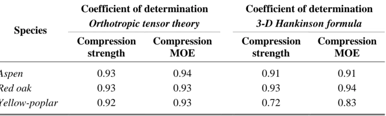
6.6 Coefficients of determination provided by the two prediction models for compression strength and MOE ... 74

6.7 Summary statistics of the experimentally determined dynamic MOE values. (Values are in GPa)... 88

6.8 Average absolute percent bias (AAPB) values associated with the three models... 93

6.9 Parameters of the first and second order regression equations, and the associated r² values ... 99

6.10 Summary statistics of the physical properties of LVL and PSL... 102

6.11 Flatwise and edgewise bending MOE of LVL and PSL (N=20)... 103

6.12 Summary statistics of the experimentally determined compression strength of LVL and PSL ... 106

6.13 Coefficients of determination provided by the various prediction models ... 107

6.14 Summary statistics of the compression MOE of the two composites ... 110

6.15 Summary statistics of the thickness of veneer sheets manufactured from the different species. (Thickness values are in mm)... 111

6.16 Summary statistics of the geometric parameters of LVL ... 114

6.17 Summary statistics of the geometric parameters of PSL... 116

7.1 Simulated geometric and physical properties of LVL and PSL (experimental LVL thickness statistics are also included) ... 129

7.2 Simulated edgewise and flatwise MOE of LVL and PSL ... 133

7.3 Simulated compression MOE of LVL and PSL in six directions... 136

7.4 The eight layup combinations; average edgewise and flatwise MOE... 139

L

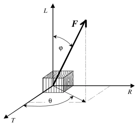
4.1 The orthotropy of solid wood shown in the principal material and global

coordinate systems. Interpretation of grain angle (ϕ) and ring angle (θ) ... 24

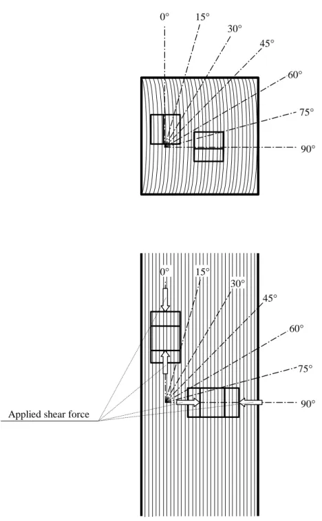
4.2 The applied shear forces in the principal anatomical planes and the notation of corresponding shear stresses. a, b – traditional shear tests, parallel to the grain; c, d – rolling shear... 26

4.3 Interpretation and principle of the prediction process of the combined models ... 31

4.4 Internal force conditions of an oblique specimen under compression ... 32

4.5 Interpretation of grain angle (ϕ) and ring orientation (θ) of the applied compression load ... 33

5.1 Dimensions of the double-notched shear specimens ... 44

5.2 Schematic of the specimen manufacturing practice from prepared, straight- grained blanks... 45

5.3 Schematic of the shear testing apparatus and the experimental setup ... 46

5.4 Compression specimen manufacturing practice and the interpretation of ϕ and θ... 47

5.5 Compression force application and the two-sided strain measurements ... 48

5.6 Schematic of the ultrasonic testing equipment and the experimental setup ... 50

5.7 Operation principle of the ultrasonic timer... 51

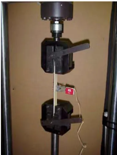
5.8 Schematic of the static tension test and the experimental setup... 53

5.9 The definition of orthogonal axes in LVL and PSL ... 57

5.10 Experimental setup of the composite bending tests... 58

5.11 Geometric structure and stochastic parameters of LVL (a) and PSL (b) ... 63

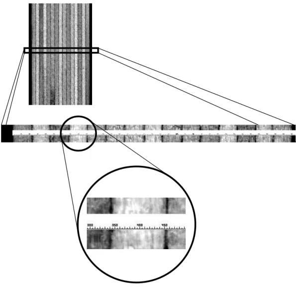
5.12 Digital images used for layer thickness measurements ... 64

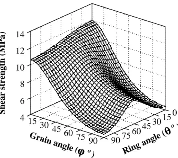
6.1 Comparison of experimental and model predicted shear strength data of quaking aspen by orthotropic diagrams... 70 6.2 Comparison of experimental and model predicted shear strength data of

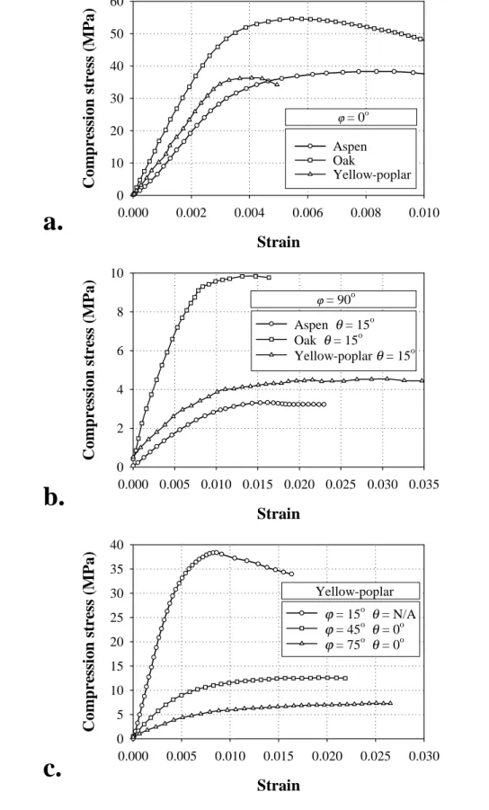
6.4 Typical stress-strain diagrams

a. Traditional, parallel to the grain compression b. Perpendicular to the grain compression

c. The effect of grain orientation ... 79

6.5 Orthotropic diagrams of compression strength and elasticity – quaking aspen... 81

6.6 Orthotropic diagrams of compression strength and elasticity – red oak... 82

6.7 Orthotropic diagrams of compression strength and elasticity – yellow-poplar... 83

6.8 Characteristic failure modes of compression specimens ... 85

6.9 Likelihood of shear failure in compression specimens a. – critical shear stress contour of specimen ϕ = 45°, θ = 15°; σu = 23.24 MPa b. – critical shear stress contour of specimen ϕ = 90°, θ = 45°; σu = 9.77 MPa .... 86

6.10 Orthotropic dynamic MOE of quaking aspen structural veneer sheets a. – experimental and model predicted values b. – Average Absolute Percentage Bias associated with the different models... 89

6.11 Orthotropic dynamic MOE of red oak structural veneer sheets a. – experimental and model predicted values b. – Average Absolute Percentage Bias associated with the different models... 90

6.12 Orthotropic dynamic MOE of yellow-poplar structural veneer sheets a. – experimental and model predicted values b. – Average Absolute Percentage Bias associated with the different models... 91

6.13 Linear (a) and quadratic (b) relationship between the static and dynamic MOE of the three Appalachian species measured at various grain angles ... 95

6.14 Relationship between dynamic MOE increase and densification for aspen (a), red oak (b) and yellow-poplar (c)... 98

6.15 Relationship between the static MOE increase and densification for yellow-poplar veneer strands with longitudinal grain orientation... 101

6.16 Comparison of the static and dynamic densification curve of yellow-poplar. Modified dynamic densification curve ... 101

6.17 Relationship between the edgewise and flatwise bending MOE of LVL (a) and PSL (b)... 104

6.18 Orthotropic diagrams of the shear strength of LVL and PSL... 108

6.19 Statistical distribution and probability density function of the veneer thickness for the three species ... 112

6.20 Layer thickness distribution throughout the thickness of LVL ... 114

6.21 Statistical distribution and probability density function of the geometric

parameters of LVL... 115

6.22 Statistical distribution and probability density function of the geometric parameters of PSL ... 117

7.1 The systematic arrangement of the strands in PSL... 121

7.2 Strands situated at various positions in a PSL cross-section ... 123

7.3 Experimental and simulated cross-sections of LVL (a) and PSL (b)... 131

7.4 Comparison of the experimental and simulated flatwise and edgewise bending MOE of LVL and PSL... 133

7.5 Comparison of the experimental and simulated compression MOE of LVL and PSL in the six simulated direction ... 136

7.6 Orthotropy diagrams created from the experimental and simulated compression MOE of the composite materials... 137

7.7 Flatwise and edgewise bending MOE of simulated LVL beams with various layups... 139

7.8 The effect of the variance of α and β on the flatwise (a) and edgewise (b) bending MOE of PSL ... 142

L

b₀ - y-intercept in polynomial functions b₁ - coefficient of x in polynomial functions b2 - coefficient of x² in polynomial functions l - longitudinal axis of a strand

n - power in the modified Hankinson formula m - angle resolution for orthotropic investigations o - cross-sectional orientation axis of a strand r² - coefficient of determination

s - standard deviation

to - original veneer/strand thickness t - layer or projected strand thickness

v - propagation velocity of sound in a material u - number of strands per in² of cross section in PSL x - longitudinal direction in the composite lumber

y - the cross-sectional direction parallel with the constitution orientation in composite lumber

z - the cross-sectional direction perpendicular to the constitution orientation in composite lumber

A - cross-section of a simulated composite beam

A_i - cross-section of a constituent in a simulated composite beam E - Modulus of Elasticity (MOE)

E - mean MOE value Eˆ - predicted MOE value Eedge - Edgewise bending MOE Eflat - Flatwise bending MOE

E_i - simulated MOE of the i^th constituent in LVL or PSL ΕI - MOE in an anatomical direction (I = L,R,T)

j

Ei - MOE measured at ϕ = i ; θ = j

ED - dynamic MOE

Ed - MOE after densification E_o - original MOE

ES - static MOE

∆E - MOE increase

I - 2^nd order moment of inertia of a beam

I_i - 2^nd order moment of inertia of a constituent around the beam’s neutral axis K - empirical constant in the three-dimensional Hankinson formula

L - longitudinal anatomical direction N - sample size

R - radial anatomical direction SSE - error sum of squares SST - total sum of squares

T - tangential anatomical direction

V - volume of a simulated composite beam section Vi - volume of a constituent in LVL or PSL

α, α1, α2 - shape parameters of a probability density function α - strand angle

β - strand deviation

δ - distance between crushed lap joints in LVL ϕ - grain angle

ϕ’ - load orientation

λ - length of crushed lap joints in LVL

µ - location parameter of a probability density function θ - ring angle

θ’ - strand/layer orientation ρ - weight density

σ - shape parameter of a probability density function σ - normal stress or strength

σ - mean normal strength value σ^ˆ - predicted normal strength value

σI - normal strength in an anatomical direction (I = L,R,T)

j

σi - normal strength measured at ϕ = i ; θ = j σmax, σu - ultimate normal stress (normal strength) τ - shear stress or strength

τ - mean shear strength value τ^ˆ - predicted shear strength value

τIJ - shear strength measured in a plane perpendicular to I, with shear loads acting in the direction J (I = R,T ; J = L,T)

j

τi - shear strength measured at ϕ = i ; θ = j τmax - ultimate shear stress (shear strength) υ - poisson ratio

ϑ - grain angle relative to the direction of internal shear stresses in compression specimens

Θ - ring angle relative to the examined sheared plane in compression specimens

AAPB - Average Absolute Percentage Bias ANOVA - Analysis of Variance

ASTM - American Society for Testing and Materials HDD - Horizontal Density Distribution

LSL - Laminated Strand Lumber LVL - Laminated Vener Lumber MC - Moisture Content

MOE - Modulus of Elasticity MSS - Maximum Shear Strength MTS - Material Testing Systems ^® PLV - Parallel Laminated Veneer PSL - Parallel Strand Lumber

PVAc - Polyvinyl Acetate

R&D - Research and Development RCB - Randomized Complete Block RH - Relative Humidity

SG - Specific Gravity STD - Standard deviation

VDD - Vertical Density Distribution

1 I

Before the 20^th century, wood was the almost exclusive building material of residential and commercial structures in North America. Abundant natural resources provided ample raw material for dams, bridges, log houses, etc. By the turn of the century the situation had changed, and the finiteness of these resources became apparent. The concept of light frame building has evolved, through balloon framing to the more contemporary platform framing used today in residential construction.

Floors and walls in light frame structures typically consist of a network of load- bearing elements (frame) covered to provide a platform surface (sheathing.) Historically, the raw material for both frame and sheathing was solid sawn lumber. In sheathing applications, wood based composite panels like plywood and – later – flakeboard, were soon substituted for solid wood. These products represent a fuller utilization of the available logs, and have other advantages in sheathing uses, such as their larger dimensions, improved uniformity of characteristics and their load-bearing capacity in two directions.

The replacement of solid wood in framing applications was more difficult. The favorable specific mechanical properties of wood make it a tough competitor for inorganic materials (steel, concrete) and wood based composite products. It was not until the last three decades of the 20^th century that the first effective composite substitute emerged in the US market. Presently, there are four types of wood based composites used for framing: Laminated Veneer Lumber (LVL), Laminated Strand Lumber (LSL) and Parallel Strand Lumber (PSL), and engineered wood I-Joists.

Although structural composite lumber products gained a substantial share of the market for construction lumber, their production cost is relatively high. Despite manufacturers' efforts, the complex production procedure and the price of adhesives used severely limit price reduction opportunities. The only feasible alternative is increasing the perceived value of these products. Manufacturers are constantly seeking alternative raw materials and innovative designs to provide superior performance and consistency at the same cost. The goal of the present study was to aid these efforts through the development of simulation models that can be used to explore new designs or raw material sources in the manufacture of composite lumber products.

1.1 Laminated Veneer Lumber (LVL)

LVL is a structural lumber manufactured from veneers laminated into a panel with the grain of all veneers running in the same direction. The resulting material is usually 19 to 45 mm (3/4 to 1-3/4 in) thick, 0.6 to 1.2 m wide, and ripped to common lumber widths of 38 to 290 mm (1-1/2 to 11-1/2 in) or wider (Wood Handbook 1999).

LVL is also known as Parallel Laminated Veneer (PLV) or Press-Lam.

The first laminated veneer structure of this type was proposed by Luxford (1944), for constructing high-strength wood aircraft members. The development of LVL for commercial use started in 1967 (Kunesh 1978.) Early studies typically used thick veneers (1/4 in or thicker) to construct and examine laminated structures (Koch 1967; FPL-Press-

sheets. The traditional raw materials for LVL manufacture are coniferous species, like Douglas-fir (Pseudotsuga mensiesii (Mirb.) Franco) and southern pine (Pinus spp.) In the 90's manufacturers started using yellow-poplar (Liriodendron tulipifera L.), too. (Vlosky et al. 1994.)

LVL has several advantages compared to solid wood lumber (based on FPL- Press-Lam Research Team 1972, Laufenberg 1983 and Vlosky et al. 1994):

• Better yield. Research has shown that "using nominal or dressed dimensions and assuming lumber recovery from the core, LVL yielded more than 47 percent more than sawn lumber" (Laufenberg 1983.) Although this is not clearly manifested in product price, this represents an environmentally sounder practice, which, through environmental marketing, can provide competitive advantage, for the producer;

• Mechanical properties. Anatomically inherent defects of solid wood (knots, sloping grain, etc.) are dispersed in LVL. This leads to increased strength and less variation in mechanical and physical properties. As a consequence, allowable stress values increase. In addition, non-destructive grading of veneers allows manufacturers to engineer the mechanical parameters of their product;

• Weight. Because of the above facts, lighter beams can be used, which speeds up construction and alleviates job site injuries;

• Size. Using a continuous process (most widespread presently), very long and deep beams can be produced at unchanged costs. The price of solid wood lumber increases with length and width, and availability of lumber is limited by the length and diameter of the saw logs;

• Reduced job site waste;

• Less frequent customer complaints.

Initially, LVL manufacturers aimed at the same market niche occupied by high quality lumber, endeavoring to keep prices competitive. In time it became apparent that LVL manufacture would remain expensive, but that the product can be superior to solid wood in many applications. Since that time, manufacturers are trying to establish their product as a value-added commodity both through R&D and marketing communication.

LVL is a relatively new product, still at the 'growth' phase of its product life-cycle.

Margins are still attractive, and production is likely to increase for a long time yet (Vlosky et al. 1994).

1.2 Parallel Strand Lumber (PSL)

PSL is a structural composite lumber made from wood strand elements with the wood fiber oriented primarily along the length of the member. The strands are coated with a waterproof structural adhesive, and fed, in a highly oriented manner, into a special press frame that uses microwave technology to cure the resin. The pressing operation results in high levels of densification. (Wood Handbook 1999)

PSL has originally developed as an alternative way of utilizing veneers that – due to defects created during growth, storage or handling – did not qualify for plywood or LVL manufacture. Its physical and mechanical properties are, however, no worse (often better) than those of LVL. Mechanical properties of PSL are just as consistent as those of LVL (Kunesh 1978, Rammer and Zahn 1997). PSL is an increasingly popular composite

The advantages and disadvantages of PSL are similar to those of LVL. Additional advantages include its appearance that many people find attractive. PSL is available in practically infinite length, while the only limitation on the cross-sectional dimension is the size of the press frame. LVL, in contrast, is typically available as 2x nominal cross- sections, or smaller.

1.3 Simulation modeling

The purpose of applied sciences is to gain better understanding of real-world facilities or processes. The traditional and most straightforward method to achieve this is experimenting with the real-life entity. In some situations, however, such investigations entail serious difficulties. Examination of real-life entities is often very costly or too disruptive to the facility or process in question. In other instances, the investigation may be very time-consuming. The subject of the examination might not even exist;

nevertheless, it might be important to study its characteristics and interaction with its hypothetical environment. In these cases, the investigator might create a simplified representation of the system to explore certain properties at lower costs, faster rates or without disrupting the original entity. This technique is called modeling.

Researchers may use various types of models, depending on the task at hand.

These include physical models, mathematical models with analytical solutions, and simulation models (Law and Kelton 1991.) Simulation models are useful if the entity to be modeled (called system) contains probabilistic elements. An example is a grocery store, where the number of customers arriving in a certain period of time, the number of

customers in the store at any time, supplies, etc. are not predictable with absolute certainty.

Wood science applications include many areas – both in material science and process control – where simulation modeling can be serviceable. In recent years, scientists employed simulation in various fields of study. These models include a wide range of applications, e.g. composite production processes (Kurse et al. 1997), hot pressing (Humprey and Bolton 1989, Lenth and Kamke 1996b), furniture rough mill operation (Anderson, 1983), laminated wood panel warping (Suchsland and McNatt 1986), etc.

Wood based composite production and properties involve many probabilistic components. Real-life experimentation with these composites, which involves altering manufacturing parameters of automated production lines, is very costly, time-consuming and disruptive. Simulation modeling is an excellent tool to investigate the manufacture, composition, physical and mechanical properties of these materials, and has been widely utilized by various researchers, as demonstrated in section 3.3.

2 O

D

S

2.1 Objectives

The objective of the research described in this dissertation was to develop and validate simulation models that can estimate the mechanical properties of Laminated Veneer Lumber (LVL) and Parallel Strand Lumber (PSL). This included the following tasks:

1. Building input databases for the model, including the orthotropic mechanical properties of the raw material and the parameters of composite geometry.

2. Examining the effect of the manufacturing process on the constituents.

3. Assessing the composites’ mechanical properties experimentally.

4. Modeling the bending and orthotropic compression Modulus of Elasticity (MOE) of the composites using deterministic and stochastic simulation, and validating the models by comparing simulation results to the experimentally obtained values.

2.2 Structure of the dissertation

Chapter 3 summarizes the results of former investigations concerning the orthotropic mechanical properties of solid wood, the effect of the manufacturing practice on the constituents and the results of simulation studies that modeled the manufacture and properties of wood based composites. Chapter 4 provides background information that was used in exploring the orthotropic nature of solid wood’s mechanical properties, and provides the theoretical basis for the simulation models.

Chapter 5 introduces the materials and experimental methods used for the investigation of the mechanical properties of solid wood and those of LVL and PSL. It also describes the practice of assessing the composites’ geometric properties that were necessary for the prediction models. The results of these investigations are discussed in Chapter 6.

Chapter 7 contains details of the developed models that predict the bending and compression MOE of the composite lumber products. This chapter includes the experimental validation of these models versus the experimentally measured properties of LVL and PSL, and demonstrates the capabilities of the models to predict the properties of composites that use alternative raw materials or design features.

Finally, chapter 8 concludes the dissertation, and chapter 9 provides recommendations for further work that might improve and extend the predictive capacity of the models.

3 L

3.1 Orthotropic strength and elasticity of solid wood 3.1.1 Orthotropy of shear strength

True shear strength is one of the most difficult characteristics to measure.

Creation of the pure shear stress state is a real challenge. Furthermore, the always present normal stresses combined with the inherent anisotropy of wood make the strength determination uncertain. Several publications have dealt with the improvement of shear strength assessment. One of the most comprehensive studies on this topic was provided by Yilinen (1963). The author investigated and critically reviewed several standardized shear testing methods. He concluded that the majority of block shear tests usually underestimate the true shear strength of solid wood.

The standard ASTM block shear test has received much criticism for not providing pure shear load on the specimens. A number of researchers addressed this problem and some also proposed alternative solutions. Norris (1957) recommended the panel shear test, and Liu (1984) suggested the adaptation of a device, proposed by Arcan et al. (1978) for wood. The drawback of these tests is that they involve complicated specimen preparation and testing procedures. Lang (1997) proposed a new device for shear strength assessment of solid wood. The advantages of the described testing apparatus are the smaller specimen size, alleviation of normal stresses and acceptable agreement with shear strength values obtained by the ASTM method.

The majority of previous research projects have focused on the shear strength of solid wood parallel to the grain. Limited publications are available that address the anisotropy of wood in shear strength assessment.

The first formula that described the strength anisotropy of wood is the well- known Hankinson’s formula (Hankinson 1921). It was developed empirically from compression tests. This equation describes the effect of grain-orientation changes on the measured properties. Many researchers examined the validity of this formula finding that it fits experimental data well (Goodman and Bodig 1972; Bodig and Jayne 1982).

However, the equation was deemed to provide adequate predictions only for compression and tension strength as well as moduli of elasticity. Kollman and Cote (1968) proposed some changes to the formula. Kollman (1934) used an experimentally determined power that provided better approximation of the direction dependent strength and elastic properties. The first attempt to describe the orthotropy of shear strength was made by Norris (1950). He applied the general Henky - von Mises theory to orthotropic materials.

Although in his study the predicted shear strength values agreed reasonably well with experimental data for structural plywood, the approach has received criticism from others (Wu 1974; Cowin 1979). Over the decades, with the advancement of man-made composites, ample research has been devoted to explore the strength and elasticity of anisotropic materials. Many of these results and theories may be applied to wood with care.

showed maximum values at approximately 15° grain orientation, rather than in the longitudinal direction. Cowin (1979) stated that a quadratic form of the Hankinson’s formula describes Ashkenazi’s data reasonably well. The proposed model, however, can not describe the shear strength maximum at 15° grain orientation. Liu and Floeter (1984) measured the shear strength of spruce at 0°, 30°, 60° and 90° grain angles with the special device described by Arcan et al. (1978) designed to provide uniform plane stress. Their results agreed well with the theory of Cowin (1979).

Some other researchers incorporated the effect of ring orientation in their works.

The experiment of Bendsten and Porter (1978) included ring-angle, but only as a blocking factor, its effect was not of interest. Okkonen and River (1989) examined the effect of radial and tangential ring orientation on the shear strength in the longitudinal direction. They concluded that Douglas-fir had higher strength when the orientation of the sheared plane was radial, while oak and maple were stronger in the tangential direction. Riyanto and Gupta (1996) tried to establish a relationship between ring angle and shear strength parallel to the grain. Using a completely randomized design, they found that ring angle had very little effect on the shear strength of Douglas-fir and Dahurian larch. Rather, the specific gravity, the percentage of latewood and the number of rings per inch were much more deterministic factors. Szalai (1994) provided an integrated approach that tackles both ring and grain angle orientation. A general equation, derived from tensor analysis, can determine the shear strength at any given ring and grain angle combination.

3.1.2 Orthotropy of compression strength and elasticity

The orthotropy of uniaxial stresses like compression and tension have received more attention than did shear stresses, both because of their ease of assessment and importance in practical applications. Much research effort was concentrated in this area, but most of the works focused on the effect of grain angle or ring angle, separately.

As mentioned in the previous section, the most well known model to describe the effect of sloping grain on compression properties is Hankinson’s formula (Hankinson 1921). Radcliffe (1965) investigated the accuracy of the equation, comparing its predictions to theoretical values of MOE that were derived from the relationships of orthtotropic elasticity. He showed that Hankinson’s solution is quite accurate in the LR plane, while in the LT plane around 25° grain inclination it may underestimate the MOE by 30%. Other researchers also verified the validity of this model (Goodman and Bodig 1972, Bodig and Jayne 1982). Kollmann and Cote (1968) suggested some modifications to the original formula, based on the results of Kollman (1934). Cowin (1979) gave a good overview of these developments, and concluded that the valid formula should be the one Hankinson originally proposed. Some published research works claimed that another version, the so-called Osgood formula, approximates better the effect of sloping grain than the Hankinson’s equation (Kim 1986, Bindzi and Samson 1995). The Osgood formula, that is also empirical, is given as follows:

(

)

(

)

q m pq

+

−

= + [3.1]

experimentally. However, no extensive validation of this model was reported in the literature (Kim 1986).

Transverse compression has received much attention, too. Bodig (1965), Kunesh (1968) and Bendsten et al. (1978) provided more in-depth analysis of the question.

Ethelington et al. (1996) incorporated variation of ring orientation in their work, and concluded that it had significant effect on the compression strength perpendicular to the grain.

The exact determination of the strength perpendicular to the grain is practically impossible because of the practical incompressibility of the wood substance. The ASTM D 143 – 83 standard requires that the test shall be discontinued after 0.1 inch crosshead- displacement. This procedure was developed to evaluate the reaction force supporting capacity of solid wood joists. Consequently, there is no standard testing method that regulates the exploration of orthotropy in compression. However, there are several theories for predicting the failure envelope of solid wood and/or wood-based composites.

Usually these approaches are based on six-dimensional tensor analyses like the Tsai-Wu strength criterion (Tsai and Wu 1971) that was developed two decades ago for homogeneous, orthotropic materials such as glass or carbon fiber and epoxy composites.

The fiber direction in these synthetic composites is better controlled and the materials are transversely isotropic (i.e., identical strength and elastic properties in any directions perpendicular to the fiber). Thus, such analyses can be successfully used in exploring the strength orthtotropy of relatively homogeneous materials as demonstrated through an analysis of paperboard by Suhling et al. (1985).

3.1.3 The orthotropy of tensile elasticity

Tensile properties of wood are more difficult to assess than compression strength and elasticity. The difficulties are even greater when sloping grain is involved. Limited research has been done on the tensile orthotropy of wood. Gerhards (1988) examined the effect of sloping grain on the tensile strength of Douglas-fir. At small angle deviations (less than 20°) he found the modified Hankinson’s formula (Kollman and Cote 1968) to provide acceptable fit. In another work (Woodward and Minor 1988) that included the full grain orientation range, the authors found the same theory to work well, but provide worse prediction than a Hyperbolic formula. Pugel (1990) developed an angle-to-grain tensile setup for thin specimens. Tensile test results of Douglas-fir and southern pine, measured using his setup, showed reasonable agreement with the original Hankinson’s formula. These studies dealt with the tensile strength only.

Nondestructive testing is a simple and inexpensive alternative to static tests. Its advantages are obvious: the specimen is not destroyed during the test, which is usually fast and cheap, and nondestructive evaluation is often much less complicated than the static test. Vibration methods are particularly suitable for quantitative, as well as qualitative evaluation of materials. The relationship of vibration properties to elastic characteristics was recognized as early as 1747 by Riccati. Researchers started to apply this relationship for wood in the early 1950’s (Pellerin 1965.)

Vibration methods include two subtypes: transverse and longitudinal (stress-

Researchers also endeavored to find empirical correlation between vibration and strength properties. Many considered the damping characteristics of wood to be promising, but experiments were not invariably successful. Pu and Tang (1997) gave an excellent overview of the research conducted in this area.

The application of static tension tests to veneers is especially limited due to their small thickness. The mechanical properties of veneer, can be very different from those of the wood it originated from, and assessment of veneer properties is sometimes desirable.

This is an area where nondestructive testing (specifically, stress-wave timing) is very helpful. There are two areas where vibration testing of veneers can be particularly useful:

1.) relating the mechanical properties of logs to those of the veneer peeled from them (Ross et al. 1999, Rippy et al. 2000), and 2.) veneer classification prior to Laminated Veneer Lumber manufacture, to engineer or improve the consistency of the product’s end properties (Koch and Woodson 1968, Jung 1982, Kimmel and Janiowak 1995, Shuppe et al. 1997.) The latter gained practical application, too, and a commercial tool is now widely used for classifying veneer sheets according to their stress-wave characteristics (Sharp 1985.)

Other studies about veneer testing by stress-waves include that of Jung (1979), who presented a comprehensive study concerning stress-wave application on veneers. He examined the potential of this technique to detect knots and slope of grain, and investigated the effect of specimen size and different measurement setups. Hunt et al.

(1989) correlated the tensile and stress-wave MOE of veneer, with acceptable results.

Most recently, Wang et al. (2001) investigated the potential of two stress-wave

techniques to detect lathe checks and knots in veneer. Stress wave propagation parameters were sensitive of defects, when measuring perpendicular to grain.

Few studies dealt with the effect of sloping grain on nondestructive testing parameters. Kaiserlik and Pellerin (1977) attempted to predict tensile strength of woods containing sloping grain. Armstrong et al. (1991) studied the effect of grain orientation on the wave-propagation velocity in various species. They concluded that, out of three equations, the modified form of the Hankinson formula (Kollman and Cote 1968) provided best fit to the data, but warned that some limitations may question its appropriateness for some applications. Divos et al. (2000) used ultrasonic propagation velocity and attenuation parameters to predict grain slope. They showed that both ultrasonic velocity and the magnitude of the first received amplitude are good indicators of grain deviation. Attenuation is better to detect small grain deviations, while propagation velocity – which is a function of the direction-dependent MOE – is a better estimator for the entire grain orientation range. Jung (1979) examined (among other factors) the effect of sloping grain on the stress-wave characteristics of veneers. He found that at small angles there is little change in stress-wave velocity, but at slightly higher orientations velocity decreases rapidly. There appears to be no study in the literature that uses vibration methods to describe the relationship between MOE and grain alignment in wood.

3.2 Modification of constituents’ properties during manufacture

The raw materials of wood based composites undergo a number of changes during processing. These effect the mechanical properties of the constituents.

Veneer peeling affects the mechanical properties of the constituents through splitting and checking on the backside of the veneer. Further modification occurs during glue application and hot pressing. Some of the adhesive applied to the constituent will penetrate its surface layer, and modify its mechanical properties.

Bodig and Jayne (1982) gave a detailed description of the phenomenon called polymeric impregnation. Based on the results of Langwig et al. (1968) and Bryant (1966) they concluded that phenolic resin tends to increase bending and compression properties, but reduce tension strength, toughness and dynamic properties. Application of the law of mixtures to impregnated wood, taking the void volume in account, yields an equation that shows that the effect of the polymer on the MOE of the compound is additive.

Experimental validation showed this theory to provide reasonable prediction for impregnated wood (Siau et al. 1968, Taneda et al. 1971).

In composite simulation, glue penetration has a double role. The more adhesive the constituents take up, the less remains for bonding. On the other hand, impregnation influences the mechanical properties, as discussed above. Triche and Hunt (1993) demonstrated the latter effect by a finite element study that incorporated a wood-resin interface layer, which increased MOE. The model predicted experimental tensile MOE and ultimate stress reasonably well.

Densification is another consequence of hot pressing. Establishing close contact between the constituents – which is imperative for good bonding – requires pressure application. The necessary pressure is higher in randomly aligned composites, and lower, but still significant in systematically aligned ones. (Dai and Steiner 1993). In either case, some densification results.

The effect of densification on mechanical properties is twofold. The original bulk of cell wall material is squeezed into a smaller volume. This means that there will be more material to resist stresses, which will improve both the strength and the elastic properties of the constituent. Xu and Suchsland (1998b) modeled the MOE of composite panels based on this assumption. According to their model, MOE improves proportionally to density-increase.

Relationships between density and MOE of solid wood seem to bear out the above theory. Bodig and Jayne (1982) presented the following equation to predict mechanical properties from density:

a b

Y = ρ , [3.2]

where Y is the characteristic in question, ρ is the density and a and b are experimental constants. Markwardt and Wilson found b to be one for bending and compression MOE.

In another study (Bodig and Goodman 1972), for the MOE of softwood and hardwood in different anatomical directions, b values differed from, but were close to, unity.

On the other hand, fractures and inelastic strains may develop within the

the effect of densification using various pressing parameters, using micromechanical tools. They concluded that high press temperatures cause less damage in the veneer, because of plastification, and are more favorable in terms of mechanical properties.

3.3 Wood composite modeling

Constituent manufacture, mat formation and consolidation are complex procedures that involve variables that, despite efforts to control them, are influenced by several random factors. The resulting products have many random characteristics, as well. It is not surprising, that many researchers used various modeling techniques to further the understanding of wood-based composites.

Modeling physical and mechanical properties requires a thorough understanding of the spatial structure of the composites. An early simulation model described the structure of paper as consisting of several layers of fibers and interfibrillar spaces or pores (Kallmes and Corte 1960, 1961). This work provided a basis to developing a mathematical model that describes randomly packed, short-fiber-type wood composites (Steiner and Dai 1993, Dai and Steiner 1994a, 1994b). This simulation is based on the observation that flake positions in a layer are driven by Poisson processes. As a consequence, point mass density and overall mat thickness will have Poisson distributions, too. The results of this investigation were used in a Monte Carlo simulation program that can model different types of mats, and analyze them for various important geometric characteristics (Lu et al. 1998). The program can also determine the effect of sampling zone size on the measured density distribution. Harris and Johnson (1982) dealt

with the characterization of flake orientation in flakeboards. They pointed out that unbounded distributions are not appropriate for this purpose and suggested a bounded distribution to provide angles between 0 and π.

Some researchers attempted to provide detailed explanation and simulate certain aspects of particle mat behavior during consolidation. Suchsland (1967) summarized the mat formation, heat- and moisture movement and stress-behavior of particleboard mats.

He provided an explanation for the formation of horizontal and vertical density distributions, and showed how pressing parameters influence the latter. Humprey and Bolton (1989) made an in-depth analysis of the multidimensional unsteady state heat and moisture transfer during hot pressing. They built a model, based on a modified finite difference approach, that could predict temperature, moisture content, vapor pressure and relative humidity in different layers of a mat.

Several works dealt with the compression behavior of flake mats throughout the pressure cycle. Dai and Steiner (1993) developed a theoretical model to describe the compression response of randomly formed wood flake mats. Their predictions agreed with experimental results reasonably well. Two further models, using somewhat different approaches to mat structure and stress-strain relationship characterization, provided improved estimation. One of these incorporated the effect of flake bending during press closure (Lang and Wolcott 1996a, 1996b) while the other used theories of cellular materials (Lenth and Kamke 1996a, 1996b.) It has been proposed that a combination of

research interest. Suchsland and Xu (1989, 1991) built physical models to examine the effect of HDD on thickness swelling and internal bond strength. They concluded that the durability of flakeboard is substantially effected by the severity of the horizontal density distribution. Xu and Steiner (1995) presented a mathematical concept for quantifying the HDD. Another study (Wang and Lam 1998) linked a simulation program with an experimental mat through a robot system that deposited flakes in the simulated positions.

Simulated and actual HDD showed good agreement.

Harless et al. (1987) created a very comprehensive simulation model that can regenerate the VDD of particleboard as a function of the manufacturing process. Other research in this area includes characterization of VDD using a trigonometric density function (Xu and Winistorfer 1996), and a simplified physical model to examine how the number of flakes, face flake moisture content and press closing time affects VDD (Song and Ellis 1997.)

Zombori (2001) created a series of linked simulation and finite element models that could, in turn, recreate the geometric structure, compression behavior, and heat and mass transfer of oriented strand board. These models could predict the inelastic stress- strain response, environmental conditions, moisture content and density at different points within the panel. His results – some of which are applicable to other composites, like particleboard, too – were in reasonable qualitative agreement with reality, although their quantitative accuracy was sometimes questionable.

Simulation studies have dealt with the mechanical properties of wood based composite panels. Most of these models were created by Xu and Suchsland. They simulated the linear expansion of particleboard (1997), followed up by a study discussing

the effect of out-of-plane orientation (1998a). In these works, they made use of the off- axis MOE, determined by the Hankinson formula. They used the findings of these studies in a later model (1998b), to simulate the uniaxial MOE of composites with uniform VDD, based on the total volumetric work. This model accounted for the effect of densification and that of particle orientation, and the authors made observations about the effect of other factors (like glueline quality and manufacturing treatments) on the simulation. Xu (1999) improved this simulation to model the effect of vertical density profile on the bending MOE of composites, using the laminate theory. He described the VDD by the trigonometric function provided by Xu and Winiesdorffer (1996), and found that maximum MOE results when peak density is some distance from the surface. The validity of this observation, however, depends on the validity of the VDD function used.

The above model was applied to evaluate the effect of percent alignment and shelling ratio on the MOE of OSB (Xu 2000) Simulation results agreed well with experimental data in literature.

Triche and Hunt (1993) modeled parallel-aligned wood strand composites using finite element analysis. They created small scale parallel-aligned strand composites, that can be regarded as physical models of LVL or PSL. The applied finite element model accounted for the effect of densification, adhesive penetration and crush-lap joints, and estimated the tensile strength and MOE of the specimens with excellent accuracy. In a very recent study, Barnes (2001) modeled the strength properties of oriented strand

agreement between experimental and model-predicted MOE, MOR and tensile strength values.

Wood based composite lumbers, such as LSL, LVL or PSL, are relatively new products that generated less research interest than did composite panels. Many findings of the above papers can be applied to these products with care. In the meantime, available literature does not seem to contain simulation studies that are directed specifically towards modeling the geometric structure and mechanical properties of these composites.

4 T

4.1 Orthotropic strength and elasticity 4.1.1 Orthotropy of shear strength

The orthotropic nature of solid wood is usually depicted in a three-dimensional Cartesian coordinate system as shown on Figure 4.1. The principal directions of the material coordinate system are noted as L, R and T, longitudinal, radial and tangential directions, respectively. If an aligned global coordinate system (xi; i=1,2,3) is

θ ϕ L(x1)

T(x )

R(x₂) x1’

x2’

systematically rotated around the R and L axes, the angles between the axes of L, R, T and xi’ (i=1,2,3) systems correspond to the grain and ring orientation of solid wood relative to the global coordinate system as marked on Figure 4.1. Note that the x1’x3’ plane is always parallel to the grain. If shear forces are acting in this plane and the direction of the applied forces is x1’, the orthotropy of shear strength can be investigated as a function of grain and ring angle. Using the described rotation, block shear specimens can be machined and tested. Such specimens are shown on Figure 4.2 representing the shear strength (τ) measurements in the principal material directions. The first subscript of τ marks the direction normal to the sheared plane while the second denotes the direction of shear forces. Specimens on Figure 4.2 a and b represent the standard shear application parallel to the grain, while shear strength measured on specimens c and d are sometimes referred to as rolling shear of solid wood.

Because of the inherent duality of shear stresses, the failure of the specimens may not manifest in the theoretically sheared plane. Furthermore, the unavoidable normal stresses may induce and propagate cracks along the weakest interface within the volume of the specimen. Such out-of-sheared-plane failure may occur with certain grain and ring angle combinations at the earlywood- latewood boundary or along the ray tissues.

Consequently, the experimentally determined values can be considered as apparent shear strength only.

Figure 4.2 – The applied shear forces in the principal anatomical planes and the notation of corresponding shear stresses. a, b – traditional shear tests, parallel to the grain;

c, d – rolling shear

τ

τ

τ

τ

a.

c. d.

b.

MODELS PREDICTING THE ORTHOTROPY OF SHEAR STRENGTH

THE ORTHOTROPIC TENSOR THEORY

In a comprehensive work Szalai (1994) used the orthotropic tensor theory to describe the direction dependent strength and elasticity of wood. Based on Ashkenazi’s (1978) strength criteria he applied a four-dimensional tensor approach to predict the shear strength of wood in any oblique plane and direction of shear forces. Substituting the tensor components with the appropriate strength values and eliminating the zero components resulting from the constraint that shear is applied only in the planes parallel to the grain, the equation takes the following form:

ϕ τ θ

ϕ τ θ

ϕ τ θ

ϕ θ τ θ

τ_ϕ^θ

2 2 2

2

2 2

2 2 2 45 90

cos 1 cos

cos 1 sin

sin 2 1 cos sin

sin 4 cos

ˆ 1

RL TL

RT

+ +

+ +

= _°

° [4.1]

where: ϕ – grain angle;

θ – ring angle;

θ

τˆϕ – estimated shear strength at grain angle ϕ and ring angle θ ;

τij – shear strength in the main anatomical planes, (i = R,T ; j = T,L) where i is the direction normal of the sheared plane and j is the direction of the applied load;

°° 45

τ90 – shear strength at 90° grain and 45° ring angle (ϕ = 90°, θ = 45°).

Note that this solution requires four experimentally predetermined strength values: three obtained in the principal anatomical planes such as τRL, τTL and τRT shown on Figure 4.2 a, b and c, respectively and a strength value at 90° grain and 45° ring angle

(τ₉₀⁴⁵_°^°). The advantages of this model are that it has a firm theoretical basis, uses only four experimentally determined data points for prediction, and is very straightforward.

QUADRATIC MODEL

Cowin (1979) demonstrated that the shear strength of wood may follow the Hankinson-type strength criterion in a quadratic form. Liu and Floeter (1984) used a tensor polynomial theory, developed by Tsai and Wu (1971), to re-derive the formula for predicting shear strength in a principal material plane of solid wood. The equation in general form is given as follows:

ϕ τ

ϕ τ

τ

τ_ϕ τ _{2 2}

90 2 2

0

2 90 2 2 0

cos sin

ˆ

°

°

°

°

= + [4.2]

where: τˆ_ϕ – estimated shear strength at grain angle ϕ ; τ 0° – shear strength at grain angle ϕ = 0°; τ 90° – shear strength at grain angle ϕ = 90°.

Like Szalai’s approach, this formula has a well-defined theoretical basis.

However, it does not include the effect of ring orientation, and has been verified experimentally in the LT plane only, using Sitka spruce specimens.

MODIFIED HANKINSON'S FORMULA

Kollman (1934) modified the original Hankinson’s formula replacing

The authors claimed that this equation provides better fit than the original Hankinson’s formula for predicting tensile strength and modulus of elasticity. Although this model is purely empirical, it has a capability to describe peak shear stresses at inclined grain, by using a higher power (i.e., n > 2). Beside the lack of theoretical basis, this model is probably very species specific and requires a significant database for accurate determination of the value of n. Like the quadratic formula, it can handle only fixed ring orientation in its present form.

COMBINED MODELS

So far, the orthotropic tensor theory was the only model that could handle both grain and ring angle changes. Researchers addressed the effect of ring orientation on the shear strength parallel to the grain and usually found it negligible. The apparent low degree of orthotropy of shear strength between the LT and LR main anatomical planes (i.e., τRL ≈ τTL) did not trigger extensive model development to describe the phenomenon.

The only available model was published by Szalai (1994). It includes two equations derived from tensor analysis, as follows:



 

 +

° =

TL

RL θτ

θτ τ^θ

2 0 2

sin cos

ˆ 1 [4.4]

τ θ τ τ

θτ θτ

τ^θ

2 4 sin

4 1 1 sin 1

cos ˆ 1

2 45

90 4

90 4



 



 − −

+ +

=

°°

°

TR RT

TR RT

[4.5]

where: τˆ – estimated shear strength at ₀^θ_° θ ring angle, ϕ = 0°;

τˆθ_90° – estimated shear strength at θ ring angle, ϕ = 90°;

and the other symbols are as given at Equation 4.1.

Equation 4.4 approximates the shear strength of traditional, parallel to the grain specimens as a function of ring orientation. It requires two experimentally predetermined strength values. The rolling shear strength variations are given by Equation 4.5 where three predetermined strength values are needed. Note that τRT and τTR represent the maximum stresses (i.e., shear strength) values. Due to the duality, the stresses in these two directions are identical. However, this is not necessarily true for the strength values of wood because of the unpredictable failure mode, as discussed earlier. Although these equations have not been experimentally verified, theoretically they should describe the effect of ring orientation on the shear strength of orthotropic materials.

One can realize that these equations can provide predetermined strength data for the quadratic model and for the modified Hankinson’s formula for predicting the effect of grain orientation. Consequently, combining Equations 4.4 and 4.5 with Equations 4.2 or 4.3, we can obtain additional two models for estimating the orthotropy of shear strength as a function of grain and ring orientation. This combination for the quadratic model is given in a short-hand form as follows:

ϕ τ

ϕ τ

τ τ_ϕ^θ _θ τ^{θ θ}_θ

2 2 90 2 2

0

2 90 2 2 0

ˆ cos ˆ sin

ˆ ˆ ˆ

°

°

°

°

= + [4.6]

Furthermore, using the modified Hankinson's formula we obtain:

ϕ τ

ϕ τ

τ

τ_ϕ^θ _{θ n}τ^{θ θ}_{θ n} cos ˆ sin ˆ

ˆ ˆ ˆ

90 0

90 0

°

°

°

°+

= [4.7]

Figure 4.3 gives a graphical explanation of these combined models. Note that both of these approximations require five experimentally predetermined strength values and Equations 4.6 or 4.7 should be solved m times where m is the resolution, calculated as m = (1 + 90/ring angle increment). During this research these two models along with the orthotropic tensor theory (Equation 4.1) were fitted to experimental data and statistically analyzed.

Figure 4.3 – Interpretation and the principle of prediction process of the combined models

0 2 4 6 8 10 12 14

15 0 45 30

75 60 90 15

30 45

60 75

90

Predicted shear strength (MPa)

Ring angle ( θ θ ^o) Grain angle (

ϕ ϕ o

)

Equation 4.4

Equation 4.5 Equation 4.6 or 4.7

τˆ₀θ_°

τˆθ_90°

°° 45

τ90

τTL

τRL

τTR

τRT