Analytic Self-Similar Solutions of the Kardar-Parisi-Zhang Interface Growing Equation with Various Noise Terms

(1)

Volume 25, Issue 2, 241–256, 2020 ISSN: 1392-6292 https://doi.org/10.3846/mma.2020.10459 eISSN: 1648-3510

Analytic Self-Similar Solutions of the Kardar-Parisi-Zhang Interface Growing Equation with Various Noise Terms

Imre F. Barna

^a

, Gabriella Bogn´ ar

^b

, Mohammed Guedda

^c

, L´ aszl´ o M´ aty´ as

^d

and Kriszti´ an Hricz´ o

^b

aWigner Research Centre for Physics

Konkoly-Thege Mikl´os ´ut 29 - 33, H-1121 Budapest, Hungary

bUniversity of Miskolc, Faculty of Mechanical Engineering and Informatics Miskolc-Egyetemv´aros 3515, Hungary

cUniversit´e de Picardie Jules Verne Amiens, Faculte de Mathematiques et d’Informatique

33, rue Saint-Leu 80039 Amiens, France

dSapientia Hungarian University of Transylvania, Faculty of Economics, Socio-Human Sciences and Engineering, Department of Bioengineering

Libert˘atii sq.1, 530104 Miercurea Ciuc, Romania E-mail(corresp.):mathk@uni-miskolc.hu E-mail:barna.imre@wigner.mta.hu

Received June 10, 2019; revised January 30, 2020; accepted January 31, 2020

Abstract. The one-dimensional Kardar-Parisi-Zhang dynamic interface growth equation with the self-similar ansatz is analyzed. As a new feature additional analytic terms are added. From the mathematical point of view, these can be considered as various noise distribution functions. Six different cases were investigated among oth- ers Gaussian, Lorentzian, white or even pink noise. Analytic solutions are evaluated and analyzed for all cases. All results are expressible with various special functions like Kummer, Heun, Whittaker or error functions showing a very rich mathematical structure with some common general characteristics.

Keywords: self-similar solution, KPZ equation, Gaussian noise, Lorentzian noise, special functions, Heun functions.

AMS Subject Classification: 35Bxx; 35Qxx; 74A50.

Copyright c2020 The Author(s). Published by VGTU Press

This is an Open Access article distributed under the terms of the Creative Commons Attribution

(2)

where u stands for the profile of the local growth [23]. The first term on the right hand side describes relaxation of the interface by a surface tension, which prefers a smooth surface. The second term is the lowest-order nonlinear term that can appear in the surface growth equation justified with the Eden model and originates from the tendency of the surface to locally grow normal to itself and has a non-equilibrium in origin. The last term is a Langevin noise to mimic the stochastic nature of any growth process and has usually a Gaussian distribution. There are numerous studies available about the KPZ equation in the literature in the last two decades. Without completeness we mention some of them. The foundation of the physics of surface growth can be found in the book of Barab´asi and Stanley [1]. Hwa and Frey [12, 17]

investigated the KPZ model with the help of the self-mode-coupling method and with renormalization group-theory, which is an exhaustive and sophisticated method using Green’s functions. They considered various dynamical scaling form of C(x, t) = x^−2ϕC(bx, b^zt) for the correlation function (where ϕ, band z are real constants). L¨assig showed how the KPZ model can be derived and investigated with field theoretical approach [22]. In a topical review paper Kriecherbauer and Krug [20] derived the KPZ model from hydrodynamical conservation equations with a general current density relation. Later, Einaxet al.[11] published a review study on cluster growth on surfaces.

Numerous models exist, which may lead to similar equations as the KPZ model, i.e., the interface growth of bacterial colonies [25]. More general interface growing models were developed based on the so-called Kuramoto-Siva- shinsky (KS) equation which is similar to the KPZ model with and extra−∇⁴u term on the right hand side of (1.1) (see [21], [36]).

Guedda has already investigated the generalized deterministic KPZ equation, when the gradient term is on an arbitrary exponent, with the self-similar ansatz [15]. Kersner and Vicsek investigated the traveling wave dynamics of the singular interface equation [19], which is closely related to he KPZ equation.

Odor and co-worker intensively examined the two dimensional KPZ equation´ with extended dynamical simulations to study the physical aging properties of different systems like glasses or polymers [18].

Beyond these continuous models based on partial differential equations (PDEs) there are numerous purely numerical methods available to study di- verse surface growth phenomena. Without completeness, we mention the ki- netic Monte Carlo [24], Lattice-Boltzmann simulations [35] and the etching model [28].

(3)

By present work, one may find certain kind of solutions to the problem [8,33]. It is already mentioned in [7] that these are for droplet initial conditions.

The first term on the right hand side of the equation can be also related to diffusion [10], and it can be found in the description of such processes [26, 27].

In this paper we analyze the solutions of the KPZ equation with the self- similar ansatz in one-dimension applying various forms of the noise term. Nu- merical results are provided both for similarity solutions with similarity variables and for the solutions with the original variables as well. The effect of the parameters involved in the problem is examined.

The similarity method is used for the investigation of analytic solution of the two dimensional Navier-Stokes equation with a non-Newtonian type of viscosity [4].

2 Theory

Non-linear PDEs has no general mathematical theory, which could help us to derive physically relevant solutions. There are different methods available, beyond the celebrated Lie algebra formalism [30] the most commonly used method is the reduction technique. This means that the original variables of the PDEs like the time t and the spatial coordinate x are used to define a new variable (e.q. ω =ω(t, x)). Via this variable transformation the original PDE can be reduced to an ordinary differential equation(ODE). The choice of the form ofω(x, t) is basically quite large. Usually, the continuity of first and second derivatives ofω in respect ofxandtis required.

Basically, there are two different trial functions (or ansatz) having well- founded physical interpretation. The first one is the traveling wave solution which mimics the wave property of the investigated phenomena described by the non-linear PDE. The second one is the self-similar ansatz of the form

u(x, t) =t^−αfx t^β

:=t^−αf(ω), (2.1)

where u(x, t) can be an arbitrary variable of a PDE and tdenotes time and x means spatial dependence. The similarity exponents α and β are of primary physical importance sinceαrepresents the rate of decay (or sharpening process ifα <0) of the magnitudeu(x, t), whileβ is the rate of spread (or contraction ifβ <0) of the space distribution fort >0. The most powerful result of this ansatz is the fundamental or Gaussian solution of the Fourier heat conduction equation (or for Fick’s diffusion equation) with α=β = 1/2. These solutions are exhibited on Figure 1 for fixed timest₁< t₂. We can generally state, that this ansatz mimics the diffusive properties (the similarities to normal diffusion) of the investigated PDE. This is the key point why this ansatz is used. We note, that in some cases [5] the traveling wave and self-similar solutions are intertwinted and can be transformed into one another.

This transformation is based on the assumption that a self-similar solution exists, i.e., every physical parameter preserves its shape during the expansion.

Self-similar solutions usually describe the asymptotic behavior of an unbounded or a far-field problem; the time t and the spacial coordinatexappear only in

(4)

Figure 1. A self-similar solution of Equation (2.1) fort1< t2. The presented curves are Gaussians for regular heat conduction.

the combination of f(x/t^β). It means that the existence of self-similar variables implies the lack of characteristic lengths and times. These solutions are usually not unique and do not take into account the initial stage of the physical expansion process. It is also transparent from (2.1) that to avoid singularity att= 0 the following transformation ˜t=t+t₀ is valid.

We should note that with the application of the Hopf-Cole transformation h=Aln(y) the non-linear KPZ equation can be converted to the regular heat conduction (or diffusion equation) with a stochastic term.

There are numerous reasonable generalizations of (2.1) available, one of them isu(x, t) =h(t)·f[x/g(t)], whereh(t) andg(t) are continuous functions.

The choice of h(t) = g(t) = √

t₀−t is a special kind, called the blow-up solution. It means that the solution becomes infinity after a well-defined finite time duration.

Gladkov [13] investigated the KPZ equation - with general exponents of the gradient term – with the self-similar blow-up solution. In a different study Gladkovet al.[14] analyzed the correctness of the KPZ equation with the same ansatz with unbounded data.

These kind of solutions describe the intermediate asymptotics of a problem. They hold when the precise initial conditions are no longer important, but before the system has reached its final steady state. For some systems it can be shown that the self-similar solution fulfills the source type (Dirac delta) initial condition. They are much simpler than the full solutions and so easier to understand and study in different regions of parameter space. A final reason for studying them is that they are solutions of a system of (ordinary differential equations (ODEs)) and they do not suffer the extra inherent numerical prob- lems related to PDEs. In some cases self-similar solutions help us to understand global physical properties of the solutions like finite oscillations, diffusion-like properties, discontinuous solutions or the existence of compact supports. Such kind of general information is hard to find from purely numerical calculations.

Applicability of this ansatz is quite wide and comes up in various mechanical systems [34], in transport phenomena like heat conduction [5], in Euler equation [6] or even in various two or three dimensional Navier-Stokes equations [2, 3].

(5)

3 Results without noise term

We start our investigation with the KPZ equation (1.1) in one spatial dimension neglecting the noise term (η(x, t) = 0). Calculating the time and spacial derivatives of (2.1) and substituting to (1.1) one gets the following constrains for the exponents: α = 0 and β = 1/2. In regular heat conduction (or diffusion) process both exponents are equal to 1/2, which means that the decay (perpendicular dynamics to the surface) and the spreading (parallel dynamics to the surface) of the solution have the same strength in time. For the KPZ equation the general features are different. Now,αvanishes, which means that we cannot identify any kind of decaying dynamics of the solution perpendicular to the surface. The non-zero value ofβ can be understood as a kind of spreading parallel to the surface. These are general and relevant statements of the surface growth process described by our solution. The remaining non-linear ODE reads

νf⁰⁰(ω) +f⁰(ω) ω

2 +λ 2f⁰(ω)

= 0. (3.1)

The general solution can be given with the logarithm of the error function f(ω) = 2ν

λln λc1

√πν erf[ω/(2√ ν)] +c2

2ν

, (3.2)

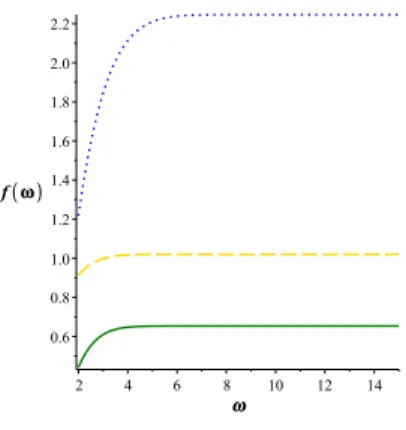
where erf is the error function [31] andc1andc2are integration constants. The role ofc2 is just a shift of the solution. For physical reasons the surface tension νshould be larger than zero. Analyzing the solution to equation (3.2), the value ofλshould be positive as well. Figure 2 presents three different shape function solutions of the ODE withc1=c2= 1 and for three different combinations of λ and ν. Note, that all solution has the same simple qualitative behavior, a quick ramp-up and a converged plateau.

Figure 3 shows the complete solutions of the original PDE showing the spatial and time dependence for c1 = c2 = λ = ν = 1. The function has a similar structure like Figure 2 a quick ramp-up and a slow convergent plateau.

We may say that different numerical values ofηandνdo not drastically change the qualitative structure of the solution surface. A closer look of the solution shows, that at t = 0 the height of the surface has a constant value, later at small times a thin valley is formed, which becomes wider and wider as time goes on. The physical parametersλ, νand the integration constants (only shifts the solutions) set the shape and the depth of the valley. Even at large times at large spatial distances, the height of the surface, i.e., the asymptotic solution remains constant. The growth of the valley (or void) can be understood as a kind of front propagation as well, and therefore can be explained with the non-zeroβ exponent.

At this point is comes clear to us, that any kind of surface growth mechanism can be only described and investigated with the additional noise term. The direct application of the self-similar solution to the KPZ equation without any additional noise termη(x, t) cannot describes any kind of growth process.

(6)

Figure 2. The self-similar solution of the KPZ equation without any noise term forc1=c2= 1. Solid line

is forλ=ν= 1, dashed line is for ν= 1 andλ= 2 and the dotted line

representsν= 2 andλ= 1.

Figure 3. The self-similar solution of the original KPZ equation without the noise term for the parameter set

c1=c2=λ=ν= 1.

4 Results with various noise terms

It is obvious that every physical process is perturbed with some kind of perturbations. Perturbations which carry no information are called noise. The KPZ equation, very correctly, includes an additive noise term. Our similarity ansatz of the form (2.1) satisfy the general ODE with the form of

νf⁰⁰(ω) +f⁰(ω) ω

2 +λ 2f⁰(ω)

+tη(ω) = 0. (4.1) If we want to apply the self-similar ansatz (2.1) to the noisy KPZ equation than the noise termtη(x, t) =l(ω) =l(x/t^β) should be some kind of analytic function of the original variables ofx, t, on the other side, we want to handle noise in a statistically correct manner,η(x, t) should be a density function of a probability distribution as well. This second condition dictates that the density function should be positive and should have an existing finite integral on a finite or infinite support. Note, the extra time dependence of the last term in (4.1) is dictated from a dimensional analysis reason.

First, we investigate noises with various power-law dependencies l(ω) = aωⁿ. Noises with different integer power values ofnare named after different colors n = −2,−1,0,1 which are brown, pink, white and blue, respectively.

Two additional cases, the Gaussian and Lorentzian noises, are investigated as well. To avoid further misunderstanding we must state that in our calculations a Gaussian noise means that the noise term explicitly depends on the scaled spatial coordinatex/t^1/2and not on the Fourier spectra as usually considered.

The argumentωof the shape function is the time-scaled spatial coordinate and not the angular frequency. Of course, in principle it is possible to evaluate the Fourier spectra of our noise terms and interpret them in the frequency domain but that is not the aim of the present study.

(7)

4.1 Brown noise n=−2

Our first case leads to the ODE of νf⁰⁰(ω) +f⁰(ω)

ω 2 +λ

2f⁰(ω)

+ a ω² = 0.

Using the mathematical program package Maple 12, the solution can be obtained in a closed form

f(ω) =−ω² 4λ+ 1

λ

ln((ω³λ²{c1M₋1

4,^d₄(r)−c2W₋1

4,^d₄(r)}²)/(M3 4,^d₄(r)

×ν·W₋1

4,^d₄(r) +M3

4,^d₄(r)·ν·d·W₋1 4,^d₄(r) + 4M₋1

4,^d₄(r)·ν·W3

4,^d₄(r))²)ν

, (4.2)

where M and W are the Whittaker M and WhittakerW functions [31]. For the better transparency we used the following notations d=√

ν²−2λa/ν for the second parameter and r = ω²/(4ν) for the argument of the Whittaker functions. Both parameters of the Whittaker functions must be real numbers, which means thatν²−2λa≥0 therefore for any kind of fixed and positive ν andλ, there is an upper limit fora, which is the strength of the noise term. So, if the magnitude of the noise reaches a definite level, the Whittaker function and the solution of the problem become undefined and meaningless. This is consistent with our physical picture about noisy processes.

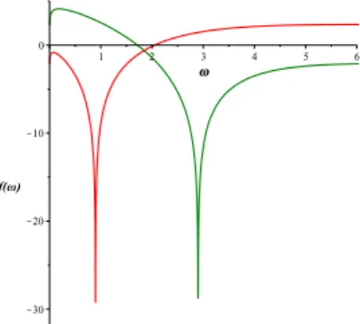
Due to the Whittaker function, the solution is undefined for negative arguments η for any kind of parameter set. Figure 4 presents the solution of equation (4.2) for two different parameter sets. The numerical value of ν defines the position of the singularity in a non trivial way, larger ν shifts the position to larger arguments. At fixed physical parameters a, ν and λ, the first integration constant c1 is equal with the asymptotic value of the solution for large arguments. The second integration constant c2 directly defines the function in the origin in a non-trivial way, the larger the value the larger the function as well.

Figure 5 shows the solution profileu(x, t) of the KPZ equation as the function of time and spatial coordinate. The sharp cusp is clearly seeing. It is also evident that the position of the cusp moves to larger spatial coordinates as time goes on, compared to the free KPZ solution of Equation (3.1), which means that the additional noise term puts a small island into the origin which is growing and pushing the cusp before. Another interesting feature is that the cusps survives even at large times and is not filled up as would we expect from our physical intuition.

The sharp but finite cusp that arises in this solutions is the so-called Van Hove singularity, which was first seen in crystals in the function of elastic frequency distribution [16]. We note, that the finite number of peaks on Figure 5 under the cusp are just an artifact of the finite resolution of the Maple software.

(8)

Figure 4. The shape functions of the Brownian noise Equation (4.2)

fora=λ= 1 ,ν= 2 physical parameters. The red line is for c1= 3, c2= 1 and and the green line

is for the integration constants c1= 1, c2= 3.

Figure 5. The solution of the KPZ equation with Brownian noise, for

the parameter set of λ=ν=c1=c2= 1 anda= 1/2.

4.2 Pink noise n=−1

The corresponding ODE reads νf⁰⁰(ω) +f⁰(ω)

ω 2 +λ

2f⁰(ω)

+ a ω = 0.

In the most general case when all three parameters are undefined (λ, ν, a), there is no closed formula available for the solution. There is an existing expression containing the integral of the HeunB functions [31] together with other functions. For given values (λ=ν =a= 1), the formula becomes a bit more transparent

f(ω) =− 1 ω²+ 2 ln

c1ω 2 H_B

1,0,−1,2,−ω 2

−c2ω 2 H_B

1,0,−1,2,−ω 2

×

(Z e^−ω²^/4

ω²HB 1,0,−1,2,^−ω₂ 2

)#

.

Unfortunately, if the strength of the noise a is different, then the term containing the integral of the functionHB cannot be separated from the pure HB function and the final form cannot be evaluated numerically.

Figure 6 shows the shape function where the physical parameters are set to unity. At first sight, the solution looks the same as the solution without noise, however there is a small positive island, which is created next to the valley. In other words the solution has a local maximum at finiteω, which means a finite time and space coordinatex/t¹². As time goes on the valley becomes wider and wider pushing this tiny island to the right with a continuous smearing. We can say that the surface growing phenomena breaks down in the dynamics of this tiny island or rather “reef”. So, there is no general surface growth phenomena along the whole axis.

(9)

Figure 7 shows the complete solution of the KPZ equation with the pink noise, note the tiny positive bump at small time and space coordinates.

Figure 6. The shape function of the pink noise fora=λ=ν= 1 and

forc1= 1 andc2= 0.

Figure 7. The complete solution of the KPZ equation for the pink noise

with the parameters given above.

4.3 White noise n= 0 The associated ODE is now

νf⁰⁰(ω) +f⁰(ω) ω

2 +λ 2f⁰(ω)

+c= 0.

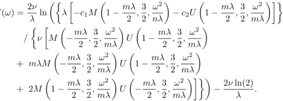
There is no general closed formula available for a general real constantc. How- ever, if the constant noise term is written in the form ofη=mλ, which can be identified as a kind of external mechanism due to the work of [9], then other analytical solutions become available which can be expressed via KummerM and Kummer U functions [31]

f(ω) =2ν λ ln

λ

−c1M

1−mλ 2 ,3

2,ω² nλ

−c2U

1−mλ 2 ,3

2, ω² mλ

/

ν

M

−mλ 2 ,3

2, ω² mλ

U

1−mλ

2 ,3 2, ω²

mλ

+ mλM

−mλ 2 ,3

2, ω² mλ

U

1−mλ

2 ,3 2, ω²

mλ

+ 2M

1−mλ 2 ,3

2, ω² mλ

U

−mλ 2 ,3

2, ω² mλ

−2νln(2) λ .

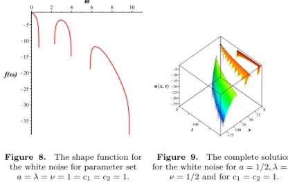
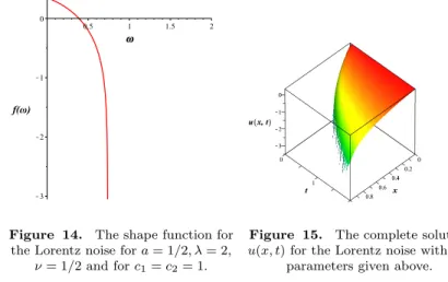
Figure 8 shows the shape function for the white noise. The new feature is that the solution fell apart to numerous distinct intervals with compact supports.

The function has large but finite negative values at the supports with infinitely large derivatives, which can be called cusps as well. Note, that there are finite intervals where the solution is not defined. Figure 9 shows the solutionu(x, t) of the KPZ equation. We mention that the separate islands continuously grow as

(10)

Figure 8. The shape function for the white noise for parameter set

a=λ=ν= 1 =c1=c2= 1.

Figure 9. The complete solution for the white noise fora= 1/2, λ= 2,

ν= 1/2 and forc1=c2= 1.

time goes on, but, they cannot touch each other even at large times. The finite number of peaks under the cusp are again an artifact of the finite resolution of the Maple software. Such kind of surface growth, where separate “barrys” are created, can be noticed on coral reefs or on dripstones.

4.4 Blue noise n= 1

The last power law noise case is the following νf⁰⁰(ω) +f⁰(ω)

ω 2 +λ

2f⁰(ω)

+aω= 0.

The structure of the solution shows some similarity to the brown and white noise and can be expressed with the help of the KummerU andM functions

f(ω) =−2ω+ 2ν/λ

×ln

( −λ(4λ−ω)

c2U(₋,¹₂, σ)−c1M(₋,¹₂, σ) 4

M(₊,¹₂, σ)U(₋,¹₂, σ)λ²+M(₋,¹₂, σ)U(₊,¹₂, σ)ν )

.

For the better transparency, we use the following notations − = −^ν+2a_2ν²^λ², + = ^ν−2a_2ν²^λ² and σ = ⁽⁴^λ−ω)_4ν ². Figure 10 presents the shape function for the blue noise. It shows some similar features to the former white noise. The solution on the positive axis can be interpreted only on two separate finite intervals. The function has finite values, however, the first derivatives at the right hand side of the intervals become infinite, which can be interpreted as a kind of “semi-cusp”. With some vertical shifts parallel to the axis f(ω) the solution can be physically interpreted as two distinct islands growing in time.

As an additional fineness, we note that at left side of the right island there is a gap.

Figure 11 shows the solution functionu(x, t) of the original PDE. The spatial range of the two distinct intervals is continuously growing in time, however,

(11)

it remains separate even at infinite times. With this kind of noise and ansatz, there is no way to grow a constant surface above the whole positive semi-axis.

Figure 10. The shape function of the blue noise for the parameter set a=λ=ν= 1 and initial conditions c1= 1 andc2= 1, respectively.

Figure 11. The complete solution u(x, t) for the blue noise with the

parameters given above.

4.5 Gaussian noise

The first non-power law noise gives us the ODE of

νf⁰⁰(ω) +f⁰(ω)0.5 [ω+λf⁰(ω)] +ae^−ω²^/n= 0.

There is no general formula available for arbitrary parameters λ, η, a and n.

Fortunately, if two parameters are fixed e.g. ν= 1/2 andn= 1, then there is a closed expression available for the solution

f(ω) =− 1 2λln

1 + tann√

λaπ·erf(p

ω/2) +c1

o2

+c2, (4.3) where erf means the error function [31]. Figure 12 presents various solutions for different values ofλ. The larger the valueλan the smaller the parametera the more the number of initial islands are, which is a remarkable new feature.

The solution itself is a continuous function on the wholeωaxis. The Van Hove singularities at finite ω are still present. Note, that at larger value of λ, the depth of the singularity valleys become shallower.

Figure 13 presents the final solution of the PDE. The general features are very similar to the formerly investigated noisea/ω²but now three independent islands increases as time goes on. The islands never grow together, the valleys stay present even at large time.

At this point we mention, that for the exponential distribution η=e^−ω/a as noise term, there is no analytic solution available at all.

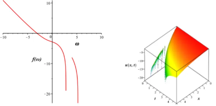
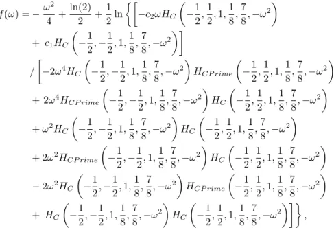
4.6 Lorentzian noise

As a last system we investigate the ODE of

νf⁰⁰(ω) +f⁰(ω)0.5 [ω+λf⁰(ω)] + a 1 +ω² = 0.

(12)

Figure 12. Various shape functions of Equation (4.3) for the

parameter set

ν= 1/2, n= 1, c2= 1 andc1= 0 for differentλvalues. Black, red and blue lines are fora= 1, λ= 25,

a= 0.25, λ= 25, and a= 0.1, λ= 55, respectively.

Figure 13. The complete solution for the Gaussian noise for

a= 0.1, λ= 55 value. Other parameters are unchanged.

Unfortunately, the general solution cannot again be given in a closed form.

In the formal solution some integrals of the confluent Heun functions remain.

For positive and given parametersν, λ, the solution becomes well-defined. As an example fora= 1/2, λ= 2 andν = 1/2, the shape function reads

f(ω) =−ω²

4 +ln(2) 2 +1

2ln

−c2ωHC

−1 2,1

2,1,1 8,7

8,−ω²

+ c1HC

−1 2,−1

2,1,1 8,7

8,−ω²

/

−2ω⁴HC

−1 2,−1

2,1,1 8,7

8,−ω²

HCP rime

−1 2,1

2,1,1 8,7

8,−ω²

+ 2ω⁴H_{CP rime}

−1 2,−1

2,1,1 8,7

8,−ω²

H_C

−1 2,1

2,1,1 8,7

8,−ω²

+ω²H_C

−1 2,−1

2,1,1 8,7

8,−ω²

H_C

−1 2,1

2,1,1 8,7

8,−ω²

+ 2ω²HCP rime

−1 2,−1

2,1,1 8,7

8,−ω²

HC

−1 2,1

2,1,1 8,7

8,−ω²

−2ω²HC

−1 2,−1

2,1,1 8,7

8,−ω²

HCP rime

−1 2,1

2,1,1 8,7

8,−ω²

+ HC

−1 2,−1

2,1,1 8,7

8,−ω²

HC

−1 2,1

2,1,1 8,7

8,−ω²

,

whereH_CandH_{CP rime}means the confluent Heun functions and the derivative of the confluent Heun function, respectively [31]. Figure 14 shows the shape function for the Lorentzian noise term. The new feature compared to the former Gaussian noise term is that the domain of the solution is just a finite interval.

(13)

Figure 14. The shape function for the Lorentz noise fora= 1/2, λ= 2,

ν= 1/2 and forc1=c2= 1.

Figure 15. The complete solution u(x, t) for the Lorentz noise with the

parameters given above.

Just a single island is born at the beginning of the surface growth process. The solution blows up (or blows down) on a finite one is the compact support of the solution. The last Figure 15 presents the final solution of the KPZ PDE. The solution has a compact support as well. It means that the small island which was positioned at the origin just grows for large times, but cannot diffuse onto the whole surface.

5 Conclusions

In summary, we can say that with an appropriate change of variables, with applying the self-similar ansatz one may obtain analytic solution for the KPZ equation for one spatial dimension with numerous noise terms. We investigated four power-law-type noisesωⁿ with exponents of−2,−1,0,1, called the brown, pink, white and blue noise, respectively. Each integer exponent describes completely different dynamics. Additionally, we investigated the properties of Gaussian and Lorentzian noises. Providing completely dissimilar surfaces with growth dynamics. All solutions can be described with non-trivial combinations of various special functions, like error, Whittaker, Kummer or Heun. The parameter dependencies of the solutions are investigated and dis- cussed. Future works are planned for the investigations of the two dimensional surfaces.

All our presented analytic formulas are in complete agreement with the statement A.B. Muravnik [29] giving a rigorous mathematical proof on absence of global positive solutions of elliptic inequalities with KPZ - nonlinearities. All the domains of our results are open sets but never the whole R axis.

We also remark that applying transformations k=e^2ν^λ^u, k =t^αm(z) and z =xt^−β to equation (1.1), one gets the linear ordinary differential equation m⁰⁰+¹₂zm⁰+ (_2ν^λtη−α)m= 0 for any arbitrary value ofαand β= 1/2.

(14)

[2] I.F. Barna. Self-similar solutions of three-dimensional Navier-Stokes equation.

Communications in Theoretical Physics,56(4):745, 2011.

[3] I.F. Barna. Self-similar analysis of various Navier-Stokes equations in two or three dimensions. In D. Campos(Ed.), Handbook on Navier-Stokes Equa- tions, Theory and Applied Analysis, New York, 2017. Nova Publishers.

https://doi.org/10.1088/0253-6102/56/4/25.

[4] I.F. Barna, G. Bogn´ar and K. Hricz´o. Self-similar analytic solution of the two-dimensional Navier-Stokes equation with a non-Newtonian type of viscosity. Mathematical Modelling and Analysis, 21(1):83–94, 2016.

https://doi.org/10.3846/13926292.2016.1136901.

[5] I.F. Barna and R. Kersner. Heat conduction: a telegraph-type model with self- similar behavior of solutions. Journal of Physics A: Mathematical and Theoret- ical,43(37):375210, 2010. https://doi.org/10.1088/1751-8113/43/37/375210.

[6] I.F. Barna and L. M´aty´as. Analytic solutions for the one-dimensional compressible Euler equation with heat conduction and with different kind of equations of state. Miskolc Mathematical Notes, 14(3):785–799, 2013.

https://doi.org/10.18514/MMN.2013.694.

[7] P. Calabrese and P.L. Doussal. Exact solution for the Kardar-Parisi-Zhang equation with flat initial conditions. Physical review letters, 106(25):250603, 2011.

https://doi.org/10.1103/PhysRevLett.106.250603.

[8] P. Calabrese, P.L. Doussal and A. Rosso. Free-energy distribution of the directed polymer at high temperature. EPL (Europhysics Letters), 90(2):20002, 2010.

https://doi.org/10.1209/0295-5075/90/20002.

[9] Z. Csah´ok, K. Honda, E. Somfai, M. Vicsek and T. Vicsek. Dynamics of surface roughening in disordered media. Physica A: Statistical Mechanics and its Appli- cations,200(1–4):136–154, 1993. https://doi.org/10.1016/0378-4371(93)90512- 3.

[10] P.L. Doussal and T. Thiery. Diffusion in time-dependent random media and the Kardar-Parisi-Zhang equation. Physical Review E, 96(1):010102, 2017.

https://doi.org/10.1103/PhysRevE.96.010102.

[11] M. Einax, W. Dieterich and P. Maass. Colloquium: Cluster growth on surfaces: Densities, size distributions, and morphologies.Reviews of modern physics, 85(3):921, 2013. https://doi.org/10.1103/RevModPhys.85.921.

[12] E. Frey, U.C. T¨auber and T. Hwa. Mode-coupling and renormalization group results for the noisy Burgers equation. Physical Review E, 53(5):4424, 1996.

(15)

[13] A. Gladkov. Self-similar blow-up solutions of the KPZ equation. International Journal of Differential Equations, 2015, 2015.

https://doi.org/10.1155/2015/572841.

[14] A. Gladkov, M. Guedda and R. Kersner. A KPZ growth model with possibly unbounded data: correctness and blow-up.Nonlinear Analysis: Theory, Methods &

Applications,68(7):2079–2091, 2008. https://doi.org/10.1016/j.na.2007.01.033.

[15] M. Guedda and R. Kersner. Self-similar solutions to the generalized deterministic KPZ equation. Nonlinear Differential Equations and Applications NoDEA, 10(1):1–13, 2003. https://doi.org/10.1007/s00030-003-1036-z.

[16] L. Van Hove. The occurrence of singularities in the elastic frequency distribution of a crystal. Physical Review, 89(6):1189, 1953.

https://doi.org/10.1103/PhysRev.89.1189.

[17] T. Hwa and E. Frey. Exact scaling function of interface growth dynamics. Physical Review A, 44(12):R7873, 1991.

https://doi.org/10.1103/PhysRevA.44.R7873.

[18] J. Kelling, G. ´Odor and S. Gemming. Suppressing correlations in massively parallel simulations of lattice models.Computer Physics Communications,220:205–

211, 2017. https://doi.org/10.1016/j.cpc.2017.07.010.

[19] R. Kersner and M. Vicsek. Travelling waves and dynamic scaling in a singular interface equation: analytic results. Journal of Physics A: Mathematical and General,30(7):2457–2465, 1997. https://doi.org/10.1088/0305-4470/30/7/024.

[20] T. Kriecherbauer and J. Krug. A pedestrian’s view on interacting particle systems, KPZ universality and random matrices. Journal of Physics A: Math- ematical and Theoretical, 43(40):403001, 2010. https://doi.org/10.1088/1751- 8113/43/40/403001.

[21] Y. Kuramoto and T. Tsuzuki. Persistent propagation of concentration waves in dissipative media far from thermal equilibrium. Progress of theoretical physics, 55(2):356–369, 1976. https://doi.org/10.1143/PTP.55.356.

[22] M. L¨assig. On growth, disorder, and field theory.Journal of physics: Condensed matter,10(44):9905, 1998. https://doi.org/10.1088/0953-8984/10/44/003.

[23] G. Parisi M. Kardar and Yi-C. Zhang. Dynamic scaling of growing interfaces.

Phys. Rev. Lett.,56:889, 1986. https://doi.org/10.1103/PhysRevLett.56.889.

[24] T. Martynec and S.H.L. Klapp. Impact of anisotropic interactions on nonequi- librium cluster growth at surfaces. Phys. Rev. E, 98:042801, Oct 2018.

[25] M. Matsushita, J. Wakita, H. Itoh, I. Rafols, T. Matsuyama, H. Sakaguchi and M. Mimura. Interface growth and pattern formation in bacterial colonies.

Physica A: Statistical Mechanics and its Applications,249(1–4):517–524, 1998.

https://doi.org/10.1016/S0378-4371(97)00511-6.

[26] L. M´aty´as and P. Gaspard. Entropy production in diffusion-reaction systems:

The reactive random Lorentz gas. Physical Review E, 71(3):036147, 2005.

[27] L. Mátyás, T. Tél and J. Vollmer. Multibaker map for shear flow and viscous heating. Physical Review E, 64(5):056106, 2001.

[28] B.A. Mello. A random rule model of surface growth. Phys- ica A: Statistical Mechanics and its Applications, 419:762–767, 2015.

https://doi.org/10.1016/j.physa.2014.10.064.

(16)

[33] T. Sasamoto and H. Spohn. One-dimensional Kardar-Parisi-Zhang equation: an exact solution and its universality.Physical review letters,104(23):230602, 2010.

https://doi.org/10.1103/PhysRevLett.104.230602.

[34] L.I. Sedov.Similarity and dimensional methods in mechanics. CRC press, 1993.

[35] D. Sergi, A. Camarano, J.M. Molina, A. Ortona and J. Narciso.

Surface growth for molten silicon infiltration into carbon millimeter- sized channels: Lattice–Boltzmann simulations, experiments and models. International Journal of Modern Physics C, 27(06):1650062, 2016.

https://doi.org/10.1142/S0129183116500625.

[36] G.I. Sivashinsky. Large cells in nonlinear Marangoni convection. Physica D: Nonlinear Phenomena, 4(2):227–235, 1982. https://doi.org/10.1016/0167- 2789(82)90063-X.