2018, No.91, 1–17; https://doi.org/10.14232/ejqtde.2018.1.91 www.math.u-szeged.hu/ejqtde/
On periodic differential equations with dissipation
Carlos A. Franco
Band Joaquin Collado
Centro de Estudios y de Estudios Avanzados del Instituto Politecnico Nacional, Mexico City 07360, Mexico
Received 31 January 2018, appeared 11 October 2018 Communicated by Alberto Cabada
Abstract. In this work we present an unexpected relation between the discriminant associated to a Hill equation with and without dissipation. We prove that by knowing the discriminant associated to a periodic differential equation, which is the summation of the monodromy matrix main diagonal entries, we are able to obtain the stability properties of damped periodic differential equation solutions. We propose to conceive the discriminant as a manifold, by doing this one can observe that the stability proper- ties of periodic differential equations are closely related to the growing rate of unstable solutions of periodic differential equations without dissipation. We show the appear- ance of the Ziegler destabilization paradox in systems of one degree of freedom. This work may be of interest for scientists and engineers dealing with parametric resonance applications or physicist working on the motion of a damped wave in a periodic media.
Keywords: periodic differential equations, stability analysis, Hamiltonian system.
2010 Mathematics Subject Classification: 34B30, 34D20.
1 Introduction
Linear differential equations with periodic coefficients have been the subject of extensive stud- ies. They can describe the dynamical behavior of a large number of mechanical systems with one or more degrees of freedom. An important second order example is the Hill equation
¨
x(t) + (α+βq(t))x(t) =0, q(t+T) =q(t), t∈ R (1.1) which has been used to describe problems in engineering and physics, including problems in mechanics, astronomy and the theory of electric circuits. Hill equation describes from the simplest systems to the more complicated ones, from a spring mass system or an L-C electric circuit up to the behavior of the suspension bridges [1] or the flow of the light in a 1D photonic crystal [18]. Hill equation often arises as a result of linearising a non-linear system about a periodic solution, for more details about the dynamical systems described by the Hill equation see [21].
It is known that periodic differential equations without dissipation have two types of so- lutions, bounded and unbounded. The type of behavior of the solutions, associated to the
BCorresponding author. Email: cfranco@ctrl.cinvestav.mx
equation (1.1), depends on the values of the parametersαandβ. The Strutt diagram or stabil- ity chart consists in dividing the plane of parametersαandβinto regions where the solutions of (1.1) are stable or unstable, see Fig. 2.2 b). The boundary curves separating stable from unstable regions are called transition curves and they are characterized by having at least one periodic solution, see [28].
In the present paper we are dealing with equations of the type (1.1) but with allowance of dissipation, that is, equations of the form
¨
x(t) +δx˙(t) + (α+βq(t))x(t) =0, q(t+T) =q(t). (1.2) If we define δ = RL and consider the capacitance as a the time varying function c(t) = α+βq(t) then (1.2) describes the charge on a series RLC network. In [5] E. Butcher and B. Mann show that a single tooth milling process may be modelled by the delay differential equation ¨x(t) +2ζx˙(t) +x(t) =−h(t) [x(t)−x(t−T)], whereh(t+T) =h(t)andζ is the damping ratio. And then, by using the system own properties, the delay differential equation is transformed into a damped periodic differential equation as in (1.2). In [17] M. Napoli et al. show that the equation (1.2) can be used to describe the dynamics of an electrostatically actuated micro-cantilever which may be used for sensing masses and as mechanical filters.
For more examples on parametric resonance see [6] and [20].
Dissipative forces are of great importance in the theory of periodic differential equations.
Generally, dissipative forces decrease unstable regions, making unstable solutions impossible for sufficiently large amount of dissipation, see [19,22,23,27]. But, there are some examples where the addition of minimum quantities of dissipation may have a destabilizing effect on the system, such phenomenon is known as Ziegler destabilization paradox [29]. This paradox was studied in depth by Bottema [2] and Kirillov [12] among many others authors; in [12]
O. N. Kirollov shows that for the Ziegler destabilization paradox to happen it is necessary the presence of both gyroscopic and dissipation forces, so the Ziegler paradox only occurs on systems with 2 or more degrees of freedom. Here we show that the paradox may also take place in systems, described by periodic differential equations, of one degree of freedom despite the absence of gyroscopic forces. Roughly speaking, the switching of a parameter, induces a gyroscopic effect, and this allows the Ziegler paradox to appear in one degree of freedom systems.
The aim of this paper is to establish the relationship between the stability analysis of a periodic differential equation with and without dissipation, in particular a Hill equation. Two unexpected effects of dissipation are described: The stability properties of both cases, systems with and without dissipation, may be obtained by knowing the so called discriminant of Hill; and the Ziegler destabilization paradox happens in systems described by a one degree of freedom Hill equation, that is, some stable solutions, of non-damped systems, become unstable after adding dissipation.
By considering the discriminant as a surface, we propose a new way to obtain the stability charts and the transition curves associated to a periodic differential equation, this also allows us to clearly exhibit the aforementioned relationship.
The work is structured as follows: in Section 2, some basic and classical properties of periodic differential equations without dissipation and some definitions are introduced; in Section 3, we study the Hill equation with dissipation case, we show that the multipliers, just as in the without dissipation case, are symmetric with respect to a circle of radiusr, we prove that the discriminant of one of the cases is the scaled discriminant of the other case and the destabilizing paradox is described.
2 Hill equation without dissipation
Consider a second order periodic differential equation
¨
y(t) + (α+βq(t))y(t) =0, α,β∈R, t∈R (2.1) where q(t)is a real periodic function q(t+T) = q(t)and ¨y = dtd22y. It is known that by the usual change of variables, z1 = y, z2 = y˙ and x = z1 z2 0
, the Hill equation (2.1) may be written as
x˙(t) =
0 1
−(α+βq(t)) 0
x(t)
, A(t)x(t). (2.2)
It is clear that, A(t+T) = A(t) and A(t) ∈ R2×2. We say that the solutions of the equation (2.2), and therefore the solutions of (2.1), are: stable if and only if they are bounded;
asymptotically stable if they tend to zero as the time tends to infinity; unstable if they tend to infinity as the time tends to infinity.
Lety1andy2 be two linearly independent solutions of (2.1) subject to the initial conditions y1(t0) =1, y2(t0) =0,
˙
y1(t0) =0, y˙2(t0) =1. (2.3) Obviously the vectors x1 = y1 y˙1 0
andx2 = y2 y˙2 0
are solutions of (2.2); moreover, the matrix Φ(t,t0) whose columns are the vectors x1 andx2 also satisfies the equation (2.2), that is
d
dtΦ(t,t0) = A(t)Φ(t,t0), Φ(t,t0) =
y1 y2
˙ y1 y˙2
.
The matrixΦ(t,t0)is known as the state transition matrix, its importance lies in the fact that it maps any solution of any linear differential equation, in particular of the system (2.2), from an initial state (initial time t0) to a final state (final timet), that is,
x(t) =Φ(t,t0)x(t0).
The state transition matrix of a periodic differential equation may be factorized as two non-singular, time dependent matrices. This factorization, maybe the most important result on the theory of periodic differential equations, it was proposed by Floquet and is stated as follows
Theorem 2.1. The state transition matrix Φ(t, 0) associated to the periodic differential equation
˙
x(t) = A(t)x(t), where A(t+T) = A(t)has the form
Φ(t, 0) =P−1(t)eRt, P(t+T) = P(t)∈R2×2, (2.4) where R is a2×2, not necessarily real matrix and P(0) = I2.
If the initial timet0is different from zero then, the factorization (2.4) takes the form Φ(t,t0) =P−1(t)eR(t−t0)P(t0), P(t+T) =P(t). (2.5)
This follows from the propertyΦ(t1,t3) =Φ(t1,t2)Φ(t2,t3). The proof of Theorem2.1 may be found in [4].
In order to show the importance of Theorem2.1, letΦ(t, 0)be the state transition matrix associated to the equation (2.2) andx(t)a solution of the same equation subject tox(0) =x0. For anyt≥0, if we writet as: t= kT+τ, whereτ∈[0,T),k is a non-negative integer andT is the minimal period ofA(t)then, the solutionx(t)can be written as
x(t) =Φ(t, 0)x0
=Φ(kT+τ, 0)x0
=Φ(kT+τ,kT)Φ(kT,(k−1)T)· · ·Φ(2T,T)Φ(T, 0)x0. By using equation (2.5) on the latter equation one gets
x(t) =Φ(τ, 0)Φ(T, 0)· · ·Φ(T, 0)Φ(T, 0)x0
=Φ(τ, 0) [Φ(T, 0)]kx0. (2.6)
From the above equation we can notice that, if we know the state transition matrix over the intervalt∈ [0,T]then, we are able to obtain any solutionx(t)at any timet.
Since the columns of Φ(t, 0) are solutions of (2.2), the matrix entries of Φ(τ, 0) are bounded; obviously the entries of the initial condition vector x0 are bounded; and the ele- ment that defines if the solutionx(t)in (2.6) tends to infinite ast→∞is[Φ(T, 0)]k. Suppose that x0 is an eigenvector of the matrix Φ(T, 0)andµi the respective eigenvalue so, it is clear that the solution (2.6) is
x(t) =µikΦ(τ, 0)x0
so the stability of the equation (2.2) solutions depends on the characteristic multipliers of the matrixΦ(T, 0). The matrixΦ(T, 0)is the well known monodromy matrix and its eigenvalues µi are known as the characteristic multipliers. From Floquet factorization, we can see that the monodromy matrix can be written as
Φ(T, 0) =eRT
where the matrixRalways can be chosen so that its eigenvaluesρi are
µi =eρiT, (2.7)
where the constantsρi are known as the characteristic exponents or Floquet exponents. Notice that the real part of the characteristic exponents defines the velocity with which the solution tends to infinity or how fast it approaches zero, this fact will be used in the next sections. The next theorem gives us the conditions for the solution of a periodic differential equation to be asymptotically stable, stable (bounded) or unstable.
Theorem 2.2. Letµi be the characteristic multipliers of the monodromy matrixΦ(T, 0)associated to the periodic differential equation x¨(t) +A(t)x(t) = 0, A(t+T) = A(t)∈ R2n×2n. Then, all the solutions are [15]:
a) asymptotically stable if and only if all|µi|<1;
b) stable (bounded) if and only if all|µi| ≤1, and if anyµi has modulo one, it must be a simple root of the minimal polynomial ofΦ(T, 0);
c) unstable if and only if there is aµisuch that|µi|>1or if all|µi|61and there is oneµj : µj
=1 andµjis a multiple root of the minimal polynomial ofΦ(T, 0).
Theorem 2.2 gives us conditions for the stability of the solutions of (2.2) in terms of the characteristic multipliersµi. So, from Theorems2.1and2.2we can conclude that the stability of solutions only depends on the knowledge of monodromy matrixΦ(T, 0).
Notice that the equation (2.2) can be written as a Hamiltonian system [16]
y˙
¨ y
=
0 1
−1 0
(α+βq(t)) 0
0 1
y
˙ y
thus, the general solution cannot be asymptotically stable, it only has two choices, to be bounded or unstable. Moreover, it is known that the state transition matrix of a Hamiltonian system is a symplectic matrix1, so the monodromy matrix is a symplectic matrix. Therefore the characteristic multipliers are symmetric with respect to the unit circle [16].
The characteristic multipliers associated to the equation (2.2) are the solutions of the char- acteristic equation
det(µI−Φ(T, 0)) =µ2−(y1(T) +y˙2(T))µ+detΦ(T, 0) =0, (2.8) where y1(t)and y2(t)are two linearly independent solutions of the Hill equation (2.1) sub- jected to the initial conditions (2.3). By Liouville’s Theorem [13] we know that the independent term in (2.8) is equal to one, that is, since Trace(A(t)) =0
detΦ(T, 0) =det(Φ(0, 0))expR0TTrace(A(τ))dτ =1.
Alternatively, the independent term is equal to one since the fact that the characteristic poly- nomial of a symplectic matrix is self-reciprocal, i.e. det(λI−Φ(T, 0)) = λ2n+p2n−1λ2n−1+ p2n−2λ2n−2+· · ·+p2n−2λ2+p2n−1λ1+1.
So, the characteristic equation is reduced to
µ2−∆(α,β)µ+1=0 (2.9)
where
∆(α,β) =y1(T) +y˙2(T). (2.10) The function ∆(α,β)is known as the discriminant associated to the Hill equation (2.1). The dependence on the coefficients α andβis written due to the dependence of the solutions on them, we will see that the discriminant plays a fundamental role in the analysis of the stability of the solutions of the equation (2.1). Solving, the characteristic equation (2.9), forµwe obtain
µ1,2= ∆(α,β)±
q∆(α,β)2−4
2 (2.11)
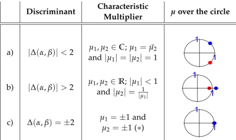
so, the characteristic multipliers µi depend on ∆(α,β) and therefore on the current value of the parametersαandβ. Table2.1shows the relation between the position of the characteristic multipliers and the discriminant associated to the Hill equation (2.1).
Following the Theorem2.2one can state the next corollary.
1We say that a matrixM∈ R2n×2nis a symplectic matrix if M0J M= J, where J is the antisymmetric matrix J=h−I0 In
n 0
i .
Discriminant Characteristic
Multiplier µ over the circle
a) |∆(α,β)|<2 µ1,µ2∈C;µ1 =µ¯2 and|µ1|= |µ2|=1
b) |∆(α,β)|>2 µ1,µ2 ∈R;|µ1|<1 and|µ2|= |1
µ1|
c) ∆(α,β) =±2 µ1 =±1 and µ2 =±1 (∗)
Table 2.1: Relation between the characteristic multipliers and the discriminant associated to (2.1). (∗) If the Jordan form of Φ(T, 0) is diagonal, then both solutions are stable; otherwise, they would be unstable.
Corollary 2.3. The solutions of the Hill equation(2.1)are:
a) stable (bounded), if |∆(α,β)| < 2, since, the multipliers are complex conjugated numbers and
|µi|=1;
b) unstable, if|∆(α,β)|> 2, since, both multipliers are real, one of them is|µ1|<1and the other is
|µ2|>1;
c) one periodic and one unstable or both periodic. If the Jordan form of the monodromy matrix is equal to the identity matrix I2 then both solutions are periodic, otherwise only one solution would be periodic.
Corollary 2.3 establishes that the stability of the equation (2.1) solutions depends on the discriminant ∆(α,β). It is known [11,15,26] that, for a fixed β = βf, the functions
∆ α,βf
±2 = 0 are entire functions of order 12, which means that they are infinitely many times differentiable functions and they have an infinite number of zerosα=αk,k=0, 1, 2, 3 . . ., the latter was proved by Haupt, see [15]. Moreover, by the fact that∆ α,βf
is an entire real function of order 12 and the Laguerre Theorem2 [25] we know that there exists an infinite number of intervalsα∈ (φ2n−1,φ2n)where ∆ α,βf
is a strictly increasing function alternat- ing with an infinite number of intervalsα∈(φ2n,φ2n+1)where∆ α,βf
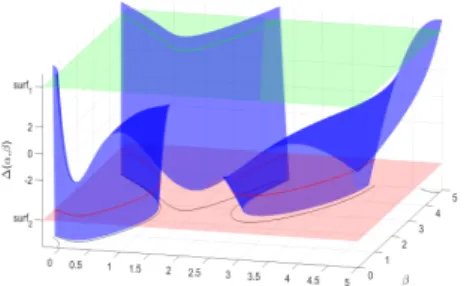
is a strictly decreasing function,n=1, 2, 3 . . . Figure2.1shows the classic form of the discriminant.
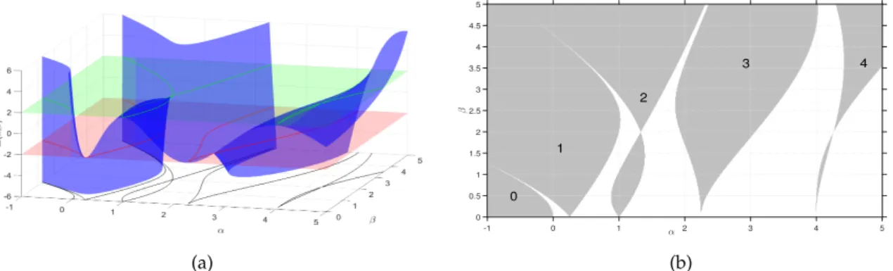
It is worth to notice that if we are able to obtain the discriminant for each point of the plane of parameters α-β, we would know the stability properties of the Hill equation solutions for each pair of parameters α and β. By continuity of the solutions we can assure that the discriminant∆(α,β)defines a surface(α,β,∆(α,β))inR3. There exist, in the literature, some discriminant approximations such as [9,10,14,24]. Moreover, if we define two parallel surfaces
2Laguerre Theorem says that if f(t)is an entire function, real for realz, of growth order less than 2 and real zeros, then the zeros ofdzd f(z)are also real and are separated from each other by the zeros of f(z).
-1 0 1 2 3 4 α 5 6 7 8 9 10
∆ (α,β)
-5 -4 -3 -2 -1 0 1 2 3 4
α0
α1
α3 α4
α5 α6
α7 α8
α9
α11
α10
α12
α2 φ2
φ3
φ4
φ5
φ6
Figure 2.1: Classical form of the discriminant∆(α,β). to theα–βplane
surf1={(α,β,z)| ∀α,β∈R,z=2}, surf2={(α,β,z)| ∀α,β∈R,z=−2}
and then, we project the intersection between the discriminant surface and surf1 and surf2, into the α–β plane, we would obtain the so called transition curves, i.e. curves that are com- posed by points, in the α–β plane, for which there is at least one periodic solution of the associated periodic differential equation, see Fig.2.2 a). The transition curves divide the α-β plane into stable and unstable zones. The unstable zones are called Arnold tongues and they are numbered from left to right; the zeroth tongue is the one more to the left, see Fig.2.2b). It can be proved that each tongue rises from the points α= nπT 2, β= 0, n= 0, 1, 2, . . ., where the numbernis the identifier of each tongue.
(a)
-1 0 1 α2 3 4 5
β
0 0.5 1 1.5 2 2.5 3 3.5 4 4.5 5
1
4 3
2
0
(b)
Figure 2.2: a) Discriminant surface (α,β,∆(α,β)). b) Stable zones in white, unstable zones in gray.
Since the determinant of the monodromy matrix Φ(T, 0) is equal to 1 we can say that Trace(R) = ρ1+ρ2 = 0, that is, det(Φ(T, 0)) = det P−1(T)eRT
but, since P(t+T) = P(t), det(P(0)) = det(P(T)) = 1. So det(Φ(T, 0)) = det eRT
= eTrace(RT) = 1, therefore Trace(RT) =0; and sinceσ(R) ={ρ1,ρ2}we can assure thatρ1+ρ2=0.
Suppose that the solutions of the system (2.2) are unstable for the pair of parameters(α,β), that is |∆(α,β)| > 2. From Theorem 2.2 if ρ1 is a characteristic exponent such that |µ1| =
eρ1T
> 1 then, ρ2 is |µ2| = |µ1|−1 = e−ρ1T
< 1. Therefore, there exists a solution which tends to infinity and one that tends to zero. The solution associated to ρ1: x1(t) = eρ1tx(0) will be exponentially unstable and the solution associated toρ2: x2(t) =eρ2tx(0) =e−ρ1tx(0)
will tend asymptotically to zero. Notice that the real part of the characteristic exponents gives us information about the solutions’ growth rate.
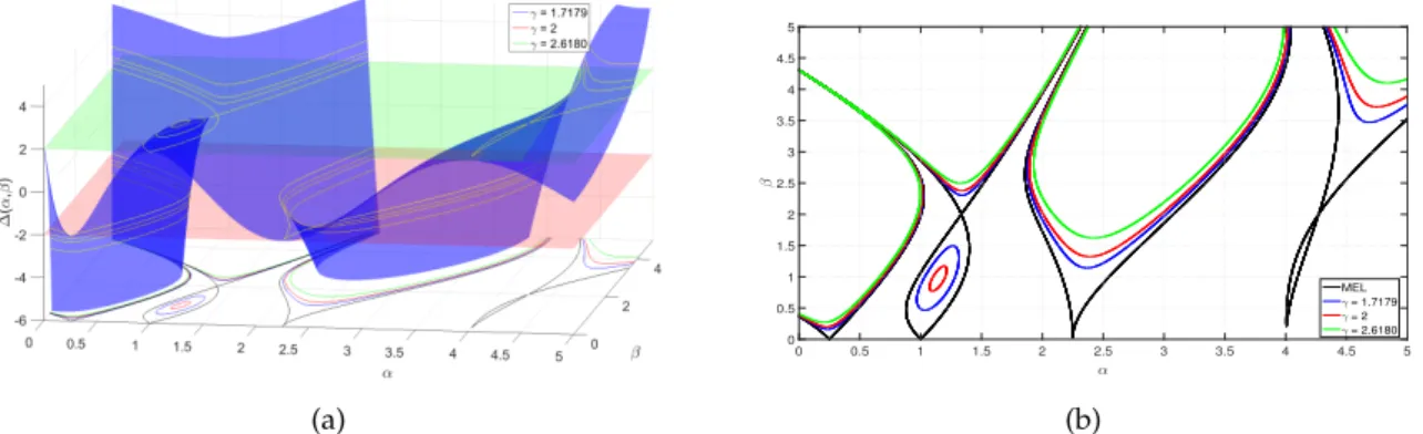
Definition 2.4. The Iso-µcurves are lines, inside the unstable zones, where the unstable solu- tion has the same growth rateγ, whereγis defined as
γ=max{|µ1|,|µ2|}=max
|µ1|, 1
|µ1|
.
From equation (2.11) we can obtain an expression of the discriminant in terms of the multipliersµ1 andµ2, that is,
∆(α,β) =µ1+µ2 =µ1+ 1
µ1 (2.12)
or, remembering the definition of characteristic exponents we have
∆(α,β) =eTρ1+eTρ2 = eTρ1+e−Tρ1 (2.13)
=2 cosh(Tρ1) (2.14)
so, from Definition2.4and the equation (2.12), we have proved a characterization of the Iso-µ curves.
Lemma 2.5. If γis as in Definition2.4 then, the Iso-µcurves are the projection, on the α-βplane, of the intersection between the surface(α,β,∆(α,β))and the planes
surfγ =
(α,β,z)| ∀α,β∈ R, z=γ+ 1 γ
, (2.15)
surf−γ =
(α,β,z)| ∀α,β∈ R, z=−
γ+ 1 γ
.
Figure 2.3 shows the Iso-µcurves over the surface (α,β,∆(α,β)) and their projection to theα–βplane.
(a)
α
0 0.5 1 1.5 2 2.5 3 3.5 4 4.5 5
β
0 0.5 1 1.5 2 2.5 3 3.5 4 4.5 5
MEL γ = 1.7179 γ = 2 γ = 2.6180
(b)
Figure 2.3: a) Discriminant Surface and its intersection with the surfaces (2.15) for several values ofγ. b) Iso-µcurves for several values ofγ.
3 Hill equation with dissipation
Adding a dissipative term to the Hill equation (2.1) we have
¨
y(t) +δy˙(t) + (α+βq(t))y(t) =0, (3.1) whereδis a non-negative real constant. By doing the same change of variables,z1 =y,z2=y˙ andx = z1 z2 0
, the Hill equation (3.1) may be written as
˙ x(t) =
0 1
−(α+βq(t)) −δ
x(t)
,Aδ(t)x(t). (3.2)
Notice that Aδ(t)is a T periodic matrix. Since the equation (3.2) is a linear equation, we are able to use Floquet’s Theorem for studying its stability. Let Φδ(t, 0) be the state transition matrix associated to (3.2). By Theorem2.2, we know that the stability of periodic differential equations depends on the position of the characteristic multipliers of the matrixΦδ(T, 0).
We know that the multipliers associated to (3.2) are the solutions of the characteristic equation
det(µiI2−Φδ(T, 0)) =µ2i −(y1(T) +y˙2(T))µi+e−δT =0, (3.3) where ∆δ(α,β)is defined as in (2.10), buty1(t)andy2(t)are linearly independent solutions of (3.1); and the linear term is equal to e−δT due to Liouville’s Theorem. Solving the equation (3.3) forµi we obtain
µi = ∆δ(α,β)± q
(∆δ(α,β))2−4e−δT
2 . (3.4)
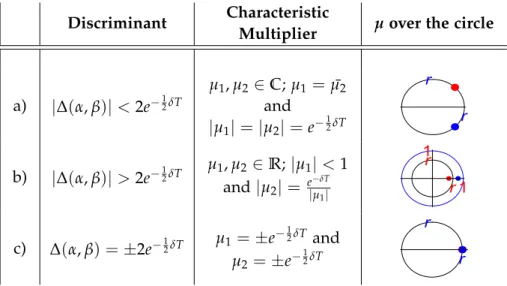
From (3.4) we can say that the multipliers are symmetric with respect to the circle of radius e−12δT. Table2.1may be re-stated as Table3.1.
Discriminant Characteristic
Multiplier µover the circle
a) |∆(α,β)|<2e−12δT
µ1,µ2 ∈C;µ1=µ¯2 and
|µ1|=|µ2|=e−12δT b) |∆(α,β)|>2e−12δT µ1,µ2∈R;|µ1|<1
and|µ2|= e|−δT
µ1|
c) ∆(α,β) =±2e−12δT µ1 =±e−12δT and µ2=±e−12δT
Table 3.1: Relation between the characteristic multipliers and the discriminant associated to (2.1).
And following Theorem2.2we get a version of Corollary2.3.
Corollary 3.1. The solutions of the Hill equation with dissipation(3.1)are:
a) asymptotically stable, if |∆δ(α,β)| < 1+e−δT, since, the multipliers are complex conjugated numbers and|µi|=e−12δT;
b) unstable, if |∆δ(α,β)|> 1+e−δT, since, both multipliers are real, one of them is|µ| <1and the other is|µ|>1;
c) one periodic and one bounded, if|∆δ(α,β)|=1+e−δT, since one multiplier is|µ|=1.
Remark 3.2. It is worth to notice that the solutions over the transition curves, associated to a Hill equation without dissipation, are usually unstable since both multipliers are equal to one or minus one but, generally they are multiple roots of the minimal polynomial, see Theorem2.2. On the other hand, the solutions of a Hill equation with dissipation, over the transition curves are always bounded, this follows from the fact that there is a multiplier equal to one (minus one) and one equal toe−δT, withδ >0.
From Corollary 3.1 we can define the transition curves of the Hill equation (3.1) as the projection of the intersection between the surface(α,β,∆δ(α,β))and the planes
surfδ1= n(α,β,z)| ∀α,β∈R, z=1+e−δTo
, (3.5)
surfδ2= n(α,β,z)| ∀α,β∈R, z=−1+e−δTo .
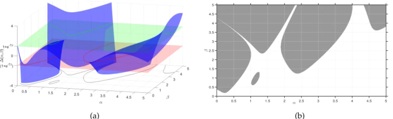
Figure 3.1 a) shows the intersection between the surface (α,β,∆δ(α,β)), associated to the equation ¨y(t) +δy˙(t) + (α+βq(t))y(t) =0, and the surfδ1 and surfδ2 planes, and Fig.3.1b) shows the stable and unstable zones, in theα–βplane, for the same equation.
(a)
0 0.5 1 1.5 2 α2.5 3 3.5 4 4.5 5
β
0 0.5 1 1.5 2 2.5 3 3.5 4 4.5 5
(b)
Figure 3.1: a) Discriminant surface associated to (3.1) and surfaces defined in (3.5), b) Stability chart associated to (3.1), stable zones in white and unstable zones in gray.
Remark 3.3. Notice that in the case of Hill equation with dissipation, the white zones, in Fig.3.1b), correspond to asymptotically stable solutions, and boundaries are characterized by having one stable (bounded) solution and one solution that tends to zero while time tends to infinity.
By adding a dissipative term to Hill equation (2.1) we have lost its Hamiltonian nature and therefore the symplectic properties are lost. On the other hand, the stable solutions of
(3.1) are not only bounded, but also they are asymptotically stable solutions and some areas that where unstable, without dissipation, became stable after adding dissipation. There are some similarities, namely: the multipliers of both systems, (2.1) and (3.1), are symmetric with respect to a circle of radius r: r = 1 for the Hill equation without dissipation (2.1); and r=e−12δT for the Hill equation with dissipation (3.1). And the stability of the solutions of both systems is determined by the current value of the discriminant ∆(α,β)(or∆δ(α,β)) at some point(α,β). In the following paragraphs we will find an unexpected relationship between the discriminants∆(α,β)and∆δ(α,β).
By doing the change of variables
y(t) =e−12δty¯(t) (3.6) one can write the Hill equation with dissipation (3.1) as a equation without dissipation, namely
¨¯
y(t) +
α− 1
4δ2+βq(t)
¯
y(t) =0. (3.7)
Now, defining
α1=α− 1
4δ2 (3.8)
and substituting (3.8) in the equation (3.7) we have
¨¯
y(t) + (α1+βq(t))y¯(t) =0. (3.9) Notice that the latter equation (3.9) has: a) the same structure as the equation (2.1), b) the same exciting functionq(t), but c) different parameterα. Therefore, the stability analysis and properties described on the first part of the present work will hold. But, remember that the solutions of the original equation (3.1) will be equal to (3.6), that is, the solutions of (3.9) will be multiplied by the decreasing functione−12δt, this multiplication is the result of adding dissipation to a Hill equation. The scalar e±12δT may be seen as a scale factor, it follows from the fact that the multipliers associated to the equation (3.9) are scaled from those associated to (3.1) by the factore12δt. The latter is proved as follows.
Define z(t) = y(t), y˙(t) 0 and ¯z(t) = y¯(t), y˙¯(t) 0. Let Φy(t,t0) and Φy¯(t,t0) be the state transition matrices associated to (3.1) and (3.9) respectively, and set the initial conditions z0 = y(t0), y˙(t0) 0 and ¯z0 = y¯(t0), y˙¯(t0) 0 so, by theory of differential equations we have
¯
z(t) =Φy¯(t,t0)z¯0. (3.10) Sincey(t) =e−12δty¯(t), it is easy to verify that
¯
z(t) =e12δtΛz(t) whereΛ=h11 0
2δ1
i
. Therefore (3.10) can be rewritten as
z(t) =e−12δ(t−t0)Λ−1Φy¯(t,t0)Λz0
so we can say that the state transition matrix of (3.1) is similar to the scaled state transition matrix of (3.9), that is
Φy(t,t0) =Λ−1he−12δ(t−t0)Φy¯(t,t0)iΛ.
If we sett= Tandt0 =0, we obtain
Φy(T, 0) =Λ−1he−12δTΦy¯(T, 0)iΛ. (3.11) The latter implies that the spectrum ofΦy(T, 0)is equal to that of the matrix
e−12δTΦy¯(T, 0) σ Φy(T, 0) =σ
e−12δTΦy¯(T, 0). (3.12) Notice that the multipliers associated to the matrix e−12δTΦy¯(T, 0)are equal to the multi- plication of each multiplier ofΦy¯(T, 0)and the scale factore−12δT, i.e.
det
νI−e−12δTΦy¯(T, 0)=ν2−e−12δTTrace Φy¯(T, 0)ν+det
e−12δTΦy¯(T, 0)
=ν2−e−12δT∆y¯(α1,β)ν+e−δT. Equaling to zero and solving forνwe get
ν1,2= e−12δTµ1,2,
whereµ1,2 are the multipliers associated to the monodromy matrixΦy¯(T, 0)so, the equation (3.12) can be written as
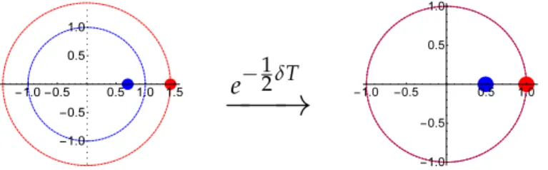
σ Φy(T, 0)=e−12δTσ Φy¯(T, 0). (3.13) Remark 3.4. Equation (3.13) shows a very interesting fact, the multipliers associated to a Hill equation with dissipation are equal to the scaled multipliers associated to a Hill equation without dissipation, i.e. the unitary circle, where the multipliers of (3.9) lie, shrinks to fit in the circle of radius r = e−12δT where the multipliers associated to the equation (3.1) lie. See Fig.3.2.
e−12δT
−−−→
Figure 3.2: The unitary circle shrinks to fit in the circle of radiusr =e−12δT.
From equation (3.11) we can obtain an even more surprising relation, by obtaining the trace to the matrices on both sides and using the linearity and the cyclicity (Trace(ABC) = Trace(CAB)) properties we get
Trace
Φy(T, 0)=e−12δTTrace
Φy¯(T, 0) or, written in terms of the discriminants
∆δ(α,β) =e−12δT∆(α1,β), (3.14) where the coefficientα1= α−12δ2 is defined as in (3.8). From Corollary3.1we know that the critical value of|∆δ(α,β)|is 1+e−δT, that is, the stability of the solutions of the Hill equation
with dissipation (3.1) depends on whether |∆δ(α,β)| is larger or smaller than 1+e−δT. By obtaining the modulo of the right hand side of (3.14) and equaling to 1+e−δT we get the condition for the transition curves of the equation (3.1) as
e−12δT|∆(α1,β)|=1+e−δT, and solving for |∆(α1,β)|
|∆(α1,β)|=2 cosh 12δT
. (3.15)
So, if we already have the discriminant surface(α,β,∆(α,β))associated to a Hill equation (2.1), and we are interested in knowing the stability zones associated to the equation with dissipation (3.1), we can use one of the following two methods: 1) To project, into the α–β plane, the intersection of the surface and the surfaces
surf1 =(α,β,z)| ∀α,β∈R,z=2 cosh 12δT ,
surf2 =(α,β,z)| ∀α,β∈R,z=−2 cosh 12δT (3.16) and then to move the origin of the plane to the left 14δ2 units, or; 2) to move the surface (α,β,∆(α,β))to the right, that is, (α,β,∆(α,β)) → α,β,∆ α−14δ2,β
and then to project the intersection of α,β,∆ α−14δ2,β
and the surfaces (3.16) into theα–βplane. Both meth- ods are shown in Fig.3.3.
Remark 3.5. Equation (3.15) gives us a surprising relation between the stability of the Hill equation with dissipation and the discriminant associated to a Hill equation without dissipa- tion. These means that, by knowing the discriminant ∆(α,β)of (2.1), we are able to analyse not only the stability of equation (2.1) but also of the equation (3.1).
Remembering, from equation (2.14), that the discriminant of equation (2.1) is equal to two times the hyperbolic cosine of the multiplication between the characteristic exponent ρ1 and the period of the excitation function, that is
∆(α,β) =2 cosh(ρ1T)
and, as we have seen if the real part of ρ1 is greater than 0 in modulo, |Re(ρ1)| > 0, then,
|∆(α,β)| > 2 and the solutions of the system (2.1) will be unstable. From the latter equation and (3.15) it is clear that, by equaling the characteristic exponent ρ1 and 12δ, and despising the effect of α1 in (3.15), that is, not moving the origin (α,β) = (0, 0) to the left, we can say that the Iso-µcurves associated to solutions of a Hill equation without dissipation, with exponential growing equal to exp(|Re(ρ1)|), are equal to the transition curves associated to the Hill equation with dissipation (3.1), see [7]. So we can say that unstable solutions of (2.1) which have growth rate less or equal to e12δT will be stabilized by adding a dissipative term δx˙(t).
The displacement, to the right, of the surface (α,β,∆(α,β)) by the addition of dissipa- tion produces an unusual behavior of the stability zones, some areas that were characterized by having stable solutions of the equation without dissipation, became unstable areas after adding dissipation. This interesting and odd fact was first observed by Ziegler in 1952, when he noticed that the critical load of a double linked pendulum was lower when a minimum amount of dissipation was added to the links joint than when no dissipation was considered, this phenomenon is known as the Ziegler destabilization paradox. So the addition of damping caused the lost of stability. In [2] O. Bottema proved that for a general linear dynamical system
(1)
−→
α
0 0.5 1 1.5 2 2.5 3 3.5 4 4.5 5
β
0 0.5 1 1.5 2 2.5 3 3.5 4 4.5 5
Discriminant associated to a Hill equation without dissipation (2.1).
Projection of the intersection between (α,β,∆(α,β))and surf1and surf2in (3.16).
↓
(2)↓
(3)(4)
−→
α
0 0.5 1 1.5 2 2.5 3 3.5 4 4.5 5
β
0 0.5 1 1.5 2 2.5 3 3.5 4 4.5 5
Moving the surface(α,β,∆(α,β))to the left
1
4δ2units.
Transition curves associated to a Hill equation with dissipation (3.1).
Figure 3.3: 1) Project the intersection of (α,β,∆(α,β)) and surf1 and surf2 in (3.16); 2) Move the surface (α,β,∆(α,β)) to the right 14δ2 units, i.e.
(α,β,∆(α,β)) → (α,β,∆(α− 14δ2,β)); 3) Move the origin of the plane to the left 14δ2 units; 4) Project the intersection of (α,β,∆(α− 14δ2,β)) and surf1 and surf2 in (3.16).
with, at least, two degrees of freedom, in particular the Ziegler pendulum, the combination of non-conservative forces and a gyroscopic force is “fatal” for stability. In [12], Kirillov gave an excellent description of the Ziegler paradox and showed a parametrically excited physical example, with non-conservative and gyroscopic forces, where the paradox arises. In [8], the authors show that the instability paradox also occurs in one degree of freedom systems such as the Kapitsa pendulum, although there are no gyroscopic forces. As final remark we have Remark 3.6. The effect of adding dissipation to a Hill equation is: to increase stability zones in theα–βplane; the stable zones, in theα–βplane, will be associated to asymptotically stable solutions; the solutions associated to transition curves will be stable; and some small areas that used to be stable without dissipation will become unstable after the addition of dissipation, those areas are always to the right of the Arnold tongue.
4 Conclusions
We have proved that the discriminant associated to a periodic differential equation does not only give us information about the stability of its solutions and how fast the unstable solu- tions tend to infinite, but also, the discriminant gives us information about the stability of the solutions when a dissipative term is added. We have seen that the addition of dissipation
has two effects on the stability of a Hill equation, one stabilizing and one destabilizing: The former refers to the fact that the unstable solutions (of a Hill equation without dissipation) which have growth rate less or equal to e12δT are stabilized after adding a dissipative term δx˙(t), stable zones in theα–βplane enlarge and the stable solutions are not only bounded but also asymptotically stable; and, the latter refers to the fact that some areas, in theα–βplane, that used to be stable, become unstable after the addition of dissipation, i.e. the Ziegler desta- bilization paradox is found in periodic differential equations, even if the dynamical system is represented by a one degree of freedom equation.
This work may be of interest for scientists and engineers dealing with parametric resonance applications or physicists working on the motion of a damped wave in a periodic media.
The latter follows from the well known fact that the solutions of the one dimensional wave equation with periodic coefficients may depend on the linear periodic differential equation (1.1) or (1.2), see [3].
Acknowledgements
The first author, acknowledges the financial support of CONACyT and CINVESTAV
References
[1] E. Berchio, F. Gazzola, A qualitative explanation of the origin of torsional instability in suspension bridges, Nonlinear Anal. 121(2015), 54–72. https://doi.org/10.1016/j.na.
2014.10.026
[2] O. Bottema, On the stability of the equilibrium of a linear mechanical system.Z. Angew.
Math. Phys.6(1955), No. 2, 97–104.https://doi.org/10.1007/BF01607296
[3] L. Brillouin, Wave propagation in periodic structures: electric filters and crystal lattices, Courier Corporation, 2003.
[4] R. Brockett, Finite dimensional linear systems, Wiley, 1970. https://doi.org/10.1137/1.
9781611973884
[5] E. A. Butcher, B. P. Mann, Analytic bounds for instability regions in periodic systems with delay via Meissner’s equation, J. Comput. Nonlinear Dynam.7(2012), No. 1, 011004, 10 pp.https://doi.org/10.1115/1.4004468
[6] T. Fossen, H. Nijmeijer(Eds.),Parametric resonance in dynamical systems, Springer Science
& Business Media, 2012.https://doi.org/10.1007/978-1-4614-1043-0
[7] C. Franco, J. Collado, Damped Hill’s equation and iso-µ curves of a related second Hill’s equation, in:2015 IEEE 54th Annual Conference on Decision and Control (CDC), IEEE, 2015, pp. 736–740.https://doi.org/10.1109/CDC.2015.7402317
[8] C. Franco, J. Collado, Ziegler paradox and periodic coefficient differential equations, in: 12th International Conference on Electrical Engineering, Computing Science and Automatic Control (CCE), IEEE, 2015, 5 pp.https://doi.org/10.1109/ICEEE.2015.7357933
[9] C. Franco, J. Collado, A novel discriminant approximation of periodic differential equations, arXiv preprint, 2017.https://arxiv.org/abs/1709.01948
[10] H. Hochstadt, Asymptotic estimates for the Sturm–Liouville spectrum, Comm. Pure Appl. Math.14(1961), No. 4, 749–764.https://doi.org/10.1002/cpa.3160140408
[11] H. Hochstadt, Functiontheoretic properties of the discriminant of Hill’s equation,Math.
Z.82(1963), No. 3, 237–242.https://doi.org/10.1007/BF01111426
[12] O. N. Kirillov, F. Verhulst, Paradoxes of dissipation-induced destabilization or who opened Whitney’s umbrella? ZAMM Z. Angew. Math. Mech. 90(2010), No. 6, 462–488.
https://doi.org/10.1002/zamm.200900315
[13] P. Lancaster, M. Tismenetsky,The theory of matrices, Academic Press, Inc., Orlando, FL, 1985.MR792300
[14] A. M. Lyapunov, The general problem of the stability of motion, Internat. J. Control 55(1992), No. 3, 521–790.https://doi.org/10.1080/00207179208934253
[15] W. Magnus, S. Winkler,Hill’s equation, Dover Publications, 2013.
[16] K. Meyer, G. Hall, D. Offin, Introduction to Hamiltonian dynamical systems and the N- body problem, Applied Mathematical Sciences, Vol. 90, Springer, New York, 2009.https:
//doi.org/10.1007/978-0-387-09724-4_1
[17] M. Napoli, R. Baskaran, K. Turner, B. Bamieh, Understanding mechanical domain parametric resonance in microcantilevers, in: The Sixteenth Annual International Confer- ence on Micro Electro Mechanical Systems, 2003, MEMS-03 Kyoto, IEEE, 2003, pp. 169–172.
https://doi.org/10.1109/MEMSYS.2003.1189713
[18] I. Nusinsky, A. A. Hardy, Band-gap analysis of one-dimensional photonic crystals and conditions for gap closing, Phys. Rev B 73(2006), No. 12, 125104. https://doi.org/10.
1103/PhysRevB.73.125104
[19] P. Pedersen, Stability of the solutions to Mathieu–Hill equations with damping,Ing. Arch.
49(1980), 15–29. https://doi.org/10.1007/BF00536595
[20] S. Rajasekar, M. A. Sanjuan,Nonlinear resonances, Springer, 2016.https://doi.org/10.
1007/978-3-319-24886-8
[21] J. A. Richards, Analysis of periodically time-varying systems, Springer Science & Business Media, 2012.https://doi.org/10.1007/978-3-642-81873-8
[22] A. Seyranian, Resonance domains for the Hill equation with allowance for damping, Dokl. Phys.46(2001), 41–44. https://doi.org/10.1134/1.1348586
[23] A. P. Seyranian, Theory of parametric resonance: modern results, in: 2003 IEEE Inter- national Workshop on Workload Characterization, IEEE, 2003, 1052–1060. https://doi.org/
10.1109/PHYCON.2003.1237051
[24] J. Shi, A new form of discriminant for Hill equation, Ann. Differential Equations15(1999), No. 2, 191–210.MR1716215
[25] E. C. Titchmarsh,The theory of functions, Oxford University Press, 1964.
[26] P. Ungar, Stable Hill equations, Commun. Pure Appl. Math. 14(1961), 707–710. https:
//doi.org/10.1002/cpa.3160140403
[27] A. van der Burgh, An equation with a time-periodic damping coefficient: sta- bility diagram and an application, Reports of the Department of Applied Mathemat- ical Analysis, 02-07, 2002. https://repository.tudelft.nl/islandora/object/uuid%
3A2f8142ec-a0ec-4b82-aa7f-deb1c4dacbef
[28] V. Yakubovich, V. Starzhinskii, Linear differential equations with periodic coefficients. 1, 2, Wiley, New York, 1975.MR0364740
[29] H. Ziegler, Die Stabilitätskriterien der Elastomechanik (in German) [Stability criteria for elastomechanics],Ing. Arch20(1952), 49–562.https://doi.org/10.1007/BF00536796