Different Mathematical Solutions on Gas Oscillation
Ferenc Szlivka
Institute of Technology, College of Dunaújváros Táncsics Mihály u. 1, 2401 Dunaújváros, Hungary e-mail: szlivkaf@mail.duf.hu
Abstract: The mathematical description of gas-pressure oscillations excited by a piston at the end of a straight duct has been investigated in an analytical way and it has been compared to numerical solutions and measured results. Two different analytical solutions have been found in the literature in series form which have been transformed into closed form solutions showing their identity. This evaluation can significantly be simplified and the comparison of the results of the analytical and the numerical solutions are presented in this study accordingly. In the results are presented the frequency of piston is close to the resonant frequency.
Keywords: gas pressure oscillation; analytical solution; infinite series; closed form
1 Introduction
The studied geometrical model with piston movement of constant frequency at one end of a pipe and with a free stream outflow to the atmosphere at the other end is shown in Figure 1. Such unsteady oscillations inside the pipe are calculated with different mathematical approaches. E.g. if amplitude of the oscillation is considered to be sufficiently small; the mathematical model of the current physical problem is the one-dimensional wave equation with the appropriate boundary conditions. In case of large amplitudes, a substantially different mathematical model must be used because the propagation of pressure waves cannot be described correctly with the solution of the linear wave equation. In the following discussion different wave equation solutions will be shown.
Jimenez [2] investigated the numerical solution of a similar gas pressure oscillation problem. An analytical investigation for the same problem is presented by Hoffmann and Fényes [1], where the problem is solved using the same mathematical model of a partial differential equation system as well as initial and boundary conditions.
R
X=0
X=L D
A
X=0,8*L L=5 m
L =5 mA
Figure 1
Schematic diagram of the gas-pressure oscillation problem
Different analytical methods are used by Hoffmann and Fényes [1] to solve the mathematical model of the pressure wave propagation. The developed analytical solutions give the same result although they are in very different forms. The aim of this study is to present a solution of simplified form for the mathematical model of the pressure wave propagation. A closed form formula is developed from the different infinite series solutions worked out by Hoffmann and Fényes [1]. If both solutions are brought into a closed form, they can be formed also formally perfectly immediately. (That out of the momentum and mass transport equations corresponding to the physical process and continuity equation diverted mathematical model that on the velocity c(x,t) and the pressure is p(x,t) related partial differential equation system ). Some parts of the solutions was published by Szlivka [4] but in German language and only in Hungary, nevertheless it was not complete. It is shown some calculated results and comparison with other theories and measured results.
The mathematical model of the pressure wave oscillation stems from the momentum and mass transport equations of the continuous fluid. It is called in the literature as acoustic model see [5], [6].
t p a 1 x
; c x p 1 t c
2
(1)
With the appropriate initial and boundary
conditions 0
) 0 , x (
c p(x,0)p0 (2)
t sin R ) t , 0 (
c p(L,t)p0
where the meaning of the symbols are: "ρ" the density of the medium; "a=347,8 m/s" the speed of sound (constant); "p" the pressure; "R " the radius of the crankshaft; "ω " drive its circle frequency; "L" the pipe length. In the first case “l”, the rod length is infinite. In chapter 6 there will be used finite rod lengths [1]
following solution is based on the Bernoulli-Fourier-method:
0
n 2 2
n n 0
n 2 2
n n
a t x cos L
a a
cos L 2
a L a t x sin R
a t x cos L
a a
cos L 2
a L a t x sin R ) t , x ( c
(3)
0
n 2 2
n n
0
n 2 2
n n 0
a t x cos L
a a
cos L 2
a L a t x sin R a
a t x sin L
a a
cos L 2
a L a t x sin R a p ) t , x ( p
(4)
With the Laplace-transformation, the
n0 n
a x L 1 n t 2 a sin
L n 2 t x sin 1 R
) t , x (
c (5)
0 n
n
0 a
x L 1 n t 2 a sin
nL 2 t x sin 1 aR
p ) t , x (
p (6)
Where sin(t-)0if t , as well as t0 , 0.
We can see two different solutions above. One with Fourier method (3), (4), the other with Laplace-transformation (5), (6). Both can be brought into closed form in order to reach the result, which will be presented in Chapter 3 and 4.
It is to be recognized that the only difference between formula (3) and (4) is constant ‘p0’, multiplicator ‘ρa’ and sign of the second term. Therefore simplification is shown only for formula (3), which can be used for formula (4) analogically.
3 Developing the Closed Form of the Infinite Series form Derived from the Bernoulli-Fourier-Method
Formula (3) contains two separate infinite series of cosine functions which can be reformulated into closed form what can be seen in expression (15) and (16). For simpler handling, the following symbols are introduced:
a
; L L X x p ; P p a; V c L ;
t T a
0
0
n p
R D a a ; B R 2, 1 n
2
(7) and these symbols applied in expression (3)
0
n 2 2
n n
0
n 2 2
n n
X T 2 cos
cos 1 X T sin 2 B
X T 2 cos
cos 1 X T sin 2 ) B T , X ( V
(8)
The infinite series expression in equation (8) can be divided into the sum of two other infinite cosine series, which comes from Ryzhik, I. M.-Gradstein, I. S.:
Tafeln [3].
j 1 2
2 1 2
i 2
2 0 2
n 2
2
j y j cos 2
i 2 2 y i 4 cos
2 1 2
n 2
2 y 1 n 2 cos 2
(9)
where y can be both T+X or T-X, and and i;j;kand n 2
k π
Ω are integer
numbers. Multiplicator (2n+1) on the left side is an odd number. The right side consists of infinite series in eq. (9)
The following notations are introduced:
1 z 0 2 and int y N where
; z 2 N
y
1 1
1
1
(10)
y and 0 z 1 intN where
; z N
y 3 3 3 3 (11)
where int() function is the largest integer part of real value.
3
1 N
N
2
if N3 an even number and (12)
1 N N
2 1 3 if N3 is an odd number.
1
i 2
2 i 1 1 2
1
i 2
2
1 1
2
1
i 2
2
1 1 2
i 2
z i 1 cos 2 4
odd N i 2
z i N i cos 2 4
i 2
z i cos 2 4
even N
(13)
Second term at the right side of the equation (9) is substituted with expression (11) and the following formula has been received
1
j 2
2 j 3 3 2
1
j 2
2
3 3
2
1
j 2
2
3 3 2
j 2
z j 1 cos odd 2
N j 2
z j N j cos 2
j 2
z j cos even 2
N
(14)
Let us use the following equations from Tafeln [3]:
sin
z cos
2 2
1 k
z k cos
0 2
k 2 2 with 0z (15)
and
sin
z cos
2 2
1 k
z k
1 cos 2
0
k 2 2
k with z (16)
supposing that “k” is an integer number, “ “ is not an integer number, (13) and (14) can be written in a simpler form. If N1 and N3 are even numbers, we get expression (15) and if N1 and N3 are odd numbers we get expression (16), if
“z” value fulfils the above indicated conditions. If N1 is an even number inequality (17) must be valid by expression (10).
0z1 (17)
This condition is almost equivalent to expression (10). It is easy to realize that after the definition by z1 and z3 conditions of the equivalences (15) and (16) are always fulfilled.
Under the application of the previous executions, we simplify the equation (9) in case if N1 and N3 are even numbers. Expression (9) can be formulated in a substantially simplified form with the application of expression (15) and (16) with the corresponding conditions for N1 and N3
.
2 sin
cos 1 N y cos 2 1 N 2 y cos 2
sin 2 z cos 2
sin 2 z 2 cos
j
z n j cos 2
i 2
z n i cos 2 4
1 2 n 2
2 y 1 n 2 cos 2
3 1
3 1
1
j 2
2
1 1 2
i 2
2
1 0 2
n 2
2
This modification was carried out if N1 and N3 are even numbers, but rather also can be solved in all other cases, as well. After application of the relations (12), one receives the expressions:
are.
numbers odd
N and N or even, N odd, N cos If
1 N 2 y sin
are.
numbers even
3 N and 1 N or odd, 3 N even, 1 N cos If
1 N 2 y sin
3 1 3
1 1
1
Introduced the expression
2
and use in the last two expressions we get the same result for all cases of odd and even N1 and N3 numbers.
cos * N 2 1 N 2 y sin cos
1 N 2 2 y sin cos
1 N 2 y sin
cos * N 2 1 N 2 y sin cos
1 N 2 2 y sin cos
1 N 2 y sin
1 1 1
1
1 1 1
1
Using the cos sin 2
; sin
cos 2
and sin
sin;
coscos and also sin
2
sin; cos
2
cos expressions, we can get one formula from the two:
cos
1 N 2 y
*cos 1
At the end of this simplification we can write in the form of the infinite series in a closed form:
cos
1 N 2 y cos 1 2
n 2
2 y 1 n 2 cos
2 1
0
n 2
2
This formula can be used in the equation (8) if y eider T + X or T -X
cos
1 N 2 X T cos cos
1 X T sin 2 B
cos
1 N 2 X T cos cos
1 X T sin 2 ) B T , X ( V
4 1
(18)
where
2 X int T 2 N
X int T
N1 4 (19)
Using the expression in the equation (18) we can get the final form of the velocity in equation (20).
cos
N 2 2 sin N 1 N X T cos B
cos
N 2 ) 1 N ( 2 cos N N X T sin B ) T , X ( V
4 4
4
1 1
1 1
(20)
und the pressure in equation (21).
cos
N 2 2 sin N 1 N X T cos D
cos
N 2 ) 1 N ( 2 cos N N X T sin D 1 ) T , X ( P
4 4
4
1 1
1 1
(21)
0 cos
.
It is important to review whether the result fulfils the initial and boundary conditions or not (2). Next investigation is to substitute these conditions to expressions (20) and (21). We circumscribe the conditions (2) with the labels (7) into non-dimensional form to this, therefore:
l P(X,0) 0, V(X,0) 0
T
T sin B T) V(0, 0
X
1 T) P(1, 1
X
At T=0 is out of (19) it is to recognize that N1-1 and N40. In this case value of the factors sin(N1l) and sinN4 in (18) and (19) is zero, and so directly that V(X,0)0and P(X,0)1.
In X0 arises out of (19) that N1N4 used; this in (18) and with trigonometric identities transformed receives one the prescribed boundary condition:
T sin cos B
cos T Bsin cos
sin T Bsin cos
2
T cos T
B cos
cos
N sin 1 N T sin ) 1 N ( sin N
T B sin ) T , 0 (
V 1 1 1 1
In X1 is out of (19) to see, that N1N41; this in (21) set and moved together, receives one (using ):
cos
N sin 1
N T
sin 1
N T
D sin 1 ) T , 1 (
P 4 4 4
If the identity is used regarding the sum of the sinus both angle, one receives the expression:
sin T N cos
cos N D sin 1 ) T , 1 (
P 4 4
Out of (19)
2
, therefore the cosine of this expression is also zero.
1,T 1P constant, that with the desired boundary condition agrees. Expressions (20) and (21) satisfy the non-dimensional forms of the equation system (1) with which exception of the points are not where P
X,T
and V
X,T
derivable. At these places, also the original expressions (3) and (4) kink points have however.Latter is maintained only based on the record of the functions.
4 Developing the Closed Form Calculated by the Laplace-Transformation Method
Only the expression (5) of the speed is reduced - like under A - because the expression of the pressure in more by more analogy manner can be transformed.
With the labels (7), becomes (5) written:
1 1 1
1
N 0 n
n N
0 n
n N
0 n
n N
0 n
n
n 2 sin 1 2
X T cos B
n 2 cos 1 2
X T sin B
n 2 sin 1 X
T cos B
n 2 cos 1 X
T sin B ) T , X ( V
(22) where under application of the next to conditions sin
T
0 if T and0
T ; 0the equations (5) and (6), and the labels
2 X int T
; 0 Max
N1 ;
1
2 X int T
; 0 Max
N2 (23)
The meaning of that is, if T-X0;sin
T-X
cos
T-X
0and if 02 - X
T ;sin
TX-2
cos
TX-2
0 must be.The expressions with summation in (22) can be written in same manner in a simpler form. One from that, for example
N 0 n
n sin2n
1 (24)
The label introduced
2
and used into the context (22), receives one after the same conversions
N
0 n
n
N 0 n N n
0 n
n
n 2 cos n cos 1
n 2 cos n sin 1 n
2 n sin 1
(25)
The first term on the right side is always same zero, that factor (-1)n cosn in the second term yields for all “n” one, therefore Eq. (24) can write further similar:
N 0
n sin
N sin 1 N n cos
2
sin
The equivalence was taken from Tafeln [3]. If the expression
N
0 n
ncos2n
1
in the same manner is simplified, one receives the simplified form:
cos
N cos 1 N
sin
The results on the expression (22) for V(X, T) used, receives one the simplified context
sin N cos ) 1 N 2 sin(
X T cos B
sin N cos ) 1 N 2 sin(
X T sin B
sin
N cos ) 1 N X sin(
T cos B
sin
N cos ) 1 N X sin(
T sin B ) T , X ( V
2 2
2 2
1 1
1 1
(26)
Let's introduce the label N4 N2 1 and simplify like (26) under application of the well known trigonometric equivalences and
2
, therefore:
cos
N 2 2 sin N 1 N X T cos B
cos
N 2 ) 1 N ( 2 cos N N X T sin B ) T , X ( V
4 4
4
1 1
1 1
(27)
After similar simplifications, the pressure arises to
cos
N 2 2 sin N 1 N X T cos D
cos
N 2 ) 1 N ( 2 cos N N X T sin D 1 ) T , X ( P
4 4
4
1 1
1 1
(28)
0
cos and T0where
2 X int T 2 N
X int T
N1 4 .
In (23) a condition was made for N1 and N2 (N4 N2 1) that they cannot be negative. Condition that T<0 must not be made because it is out of the initial conditions. The values k do not belong to the domain of the velocity formulas (27) and pressure formulas and (28), while in the formulas (5) and (6) it belong to the definition area, however the corresponding expressions have the same limit. (When kit is the own resonance frequency of the pipe.) It is to be recognized that velocity relation and pressure relation (20) and (21) simplified with the Fourier method will match relations (27) and (28) simplified with Laplace-transformation.
The boundary conditions of the physical process were indicated through the equations (2). A fully sinusoidal excite expression was supposed on the closed end of the pipe. As equations (1) and the boundary conditions are homogeneous linear, the resulting solution can be produced as a sum of divided solutions of several sinusoidal expressions with different amplitudes and frequencies. The simplified forms have especially large advantages in these cases as in [1] indicated end formulas. The advantages arise in the simpler calculation and in the less required time duration. The next chapter is presenting a practical calculation of these results.
5 Results of Analytical and Numerical Solutions
Let us look through the gas dynamic solution of this mathematical problem. The gas dynamic model was solved with the help of method of characteristics. The differential equation system has a different form from the equation (1).
x 0 c c t
; t x 0 p 1 t c c t
c
(29)
The main difference between the two models is that the "a" value, the speed of sound is not constant in the gas dynamic model. The wave equation of gas dynamics uses the basic relations without neglect, although it is more expedient to modify the equation system in such a manner that the dependent variables in it should be the velocity c = c (x,t) and the speed of sound a = a ( x, t ). Hence
x 0 a a 1 2 t c c t
; c t 0 a 1 2 x c a 1 2 x
a c
(30)
The quasi-linear partial differential equation system is hyperbolic. The applied numerical solution is called the method of characteristics. The details are in the [2]. And there is no analytical solution for this differential equation system. At the physical plane [x, t,] along the projection of the characteristic curve with a given tangent, the correlations of the independent variables can be written in the non- dimensional form, in the well-known manner, as
; A 2 V
; 1 A 2 V
1
a0
V c
Where and are the Riemann-variables and V c/a0: the non-dimensional velocity and Aa/a0: the non-dimensional speed of sound. The isentropic change of state has been used in each case to determine pressure. The boundary condition is a little bit different, the pressure on the open end of the pipe is not constant. The details can be seen in the [5]. In Figure 2 you can see different model solutions and measured results from [7]. The calculated gas oscillation frequency 317,291/s is very close to the resonant frequency
s / 1 19 ,
r 327
.
According to Figure 2 the solution of the wave equation of acoustics has shown a difference of about l0 % less in the amplitude, related to that one of gas dynamics.
On the basis of the examinations it can be stated that the pressure patterns forming in the system are equal regarding the frequency, depending on the calculation method, but from the point of view of the pressure values, considerable differences appear, according to the preceding valuations. The analytical solution can be used to predict the gas velocity and pressure fluctuation inside a straight pipe. It is simpler to use than the gas dynamic model.
av
X
Figure 2
Comparison of the different solutions
We have some measurement results, too. The measurement data are between the acoustic and the gas dynamic model results. In the real case the friction force decreases the velocity and the pressure amplitude. For example, in the [8] J. J.
Patel and U. V. JoshI show CFD calculation results of a gas oscillation where there is friction in the pipe.
6 Some Calculated Results
The gas oscillation problem can be solved analytically not only in a clear sinusoidal excitation. It is an opportunity for the analytical solution if the piston velocity is more complicated function of time, for example when the piston rod is not infinite. The differential equation system is the same (1)
t p a2 1 x
; c x p 1 t c
(31)
The appropriate initial and boundary conditions are the next:
p0
) 0 , x ( p 0 ) 0 , x (
c
sin2ωt
2 t λ sinω Rω t)
c(0, p(L,t)p0 (32)
where the meaning of the symbols are: " " the density of the medium; "a0=347,8 m/s" the speed of sound (constant is); "p" the pressure; "R0,011m" the radius of the crankshaft; “ 0,044m“ the piston rod length; “ 0,25
R
“ the piston rod ratio; "" drive its circle frequency; "L5m" the pipe length. The velocity
) t, 0 (
c function is an approximation: the first two terms of a Taylor’s series for a finite rod length. The first term is at infinite piston rod length in the previous section.
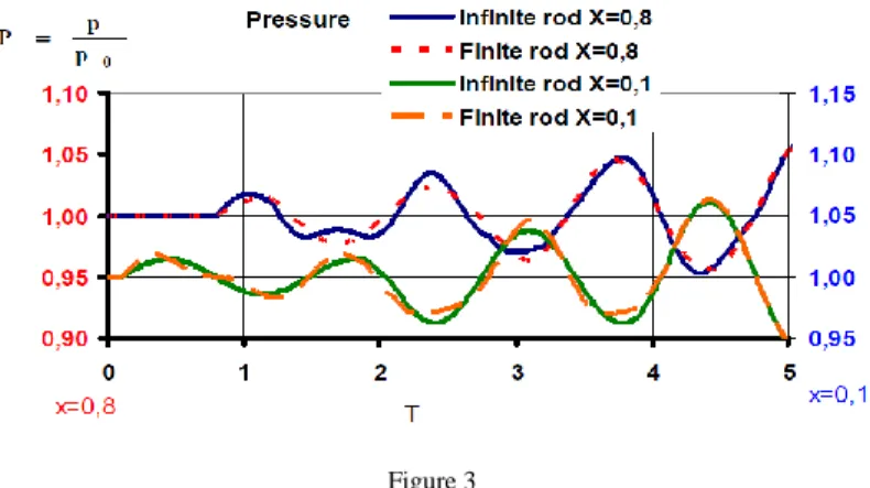
The (31) equation system is homogenious linear so the solution of a sum of two functions is the sum of the two solutions. In this case pressure and velocity oscillation were calculated. Figures 3 and 4 show the results. Non-dimensional velocity,
a0
V c and non-dimensional pressure, p0
P p )are used in the diagrams.
Figure 3 shows the pressure functions at infinite and finite piston rod while Figure 4 shows the velocity functions. Pressure and velocity functions were calculated at
2 , 0
X and X0,8 . The function is zero until the wave from the piston reaches the observation point at X0,2 or X0,8 . The difference between the finite and infinite functions is bigger until two or three oscillations. After some periods the difference can be neglected. You can see that the functions of pressure and velocity have some broken points where the functions are not derivable. It is an interesting property of the solution.
Figure 3
Comparison the pressure functions of the “infinite” and “finite” piston rod solutions (The vertical scale is shifted)
Figure 4
Comparison the velocity functions of the “infinite” and “finite” piston rod solutions (The vertical scale is shifted)
Conclusion
Two different mathematical infinite series solutions exist in the literature. In this article they were transformed out of an endless row into closed form. Both simplifying methods reached the same result as a closed form. It is simpler to use these solutions than the gas dynamic numerical simulation. The comparison with other numerical solutions and measured results shows a good agreement.
References
[1] Hoffmann, A - Fényes, T. (1982) ‘Rechenferfharen zur Unterzuchungen von Wellenerseinungen in Rohrleitungen‘ Periodika Polytechnica Mech.
Eng. 26/1 (1982) U.T. Budapest
[2] Jimenez, I. (1973) ‘Fluid Mechanics‘, Great Britain, 23
[3] Ryzhik, I. M. - Gradtein, I. S. (1957) ‘Tafeln‘, Berlin Deutscher Verlag der Wissenschaften
[4] Szlivka, F. (1983) ‘Herstellung der geschlossenen Lősung des Differentialgleichungssystems von Gasschwingungen‘, Periodica Polytechnica Mech. Eng. 27/1 (1983)
[5] Bencze, F. - Hoffmann. A. - Szlivka, F. (1983) ‘Untersuchung der Wellenerscheinungen in Rohrleitungen‘, ZAMM 63. pp. 228-231
[6] Engelhardt, J. (2012) ‘Schwingungen von Rohrleitungen aktiv mindern, Artikel aus der Zeitschrift‘ 3R Fachzeitschrift für sichere und effiziente Rohrleitungssysteme ISSN: 2191-9798. Nr. 5, 2012, Seite 396-400, Abb.
[7] Bencze, F. - Hoffmann. A. - Szlivka, F (1983) ‘Examination of Forced Gas Oscillations by the Aid of Computer‘, The Seventh Conference on Fluid Machinery, Budapest 1983. pp. 228-231
[8] J. J. Patel and U. V. JoshI (2012) ‘Study of the Oscillating Flow in the Circular Tube Using CFD‘, World Journal of Science and Technology 2012, 2(4) pp. 46-49, ISSN: 2231-2587