CHAPTER 2
Fluid Motion and Mixing
Robert S . Brodkey Department of Chemical Engineering, The Ohio State University,
Columbus, Ohio
I. Introduction 7 II. Description of Diffusion and Mixing Processes 8
A. Molecular Diffusion in Laminar Flow 8 B. Eddy Diffusion in Turbulent Flow 10
C. Bulk Diffusion 48 D. Mixing 57 III. Criteria for Mixing 61
A. Scale of Segregation 61 B. Intensity of Segregation 62
IV. Laminar Mixing 66 V. Turbulent Mixing 67
A. Isotropic Homogeneous Field 68 B. Chemical Reaction and Reactors 80 C. Nonisotropic Inhomogeneous Field 87
D. Experimental Results 92 VI. Summary and Prospectus 100
List of Symbols 1 0 2 References 105
I. Introduction
The terms "diffusion" a n d " m i x i n g " have been used to describe a multitude of physical processes, some of which occur and can be studied separately and others which exist only as groups of simultaneous processes. Before one can attempt to relate any of these processes to the fluid dynamics of a system, a visualization, upon which a mathematical model will be based, is necessary.
For this reason, the first section of this chapter will dwell u p o n a description of diffusion and mixing processes. Here, the terms will be defined, the proces- ses described, and the basic relations derived. It is hoped t h a t the reader will find that the required background material provided is adequate, but refer- ences are included to facilitate further study. Once the definitions of the various diffusion and mixing processes have been established, criteria for mixing can be presented. These criteria will be the starting point for the actual theories of mixing. Both laminar and turbulent conditions will be considered.
7
As will be seen, some progress has been made in developing satisfactory theories for predicting mixing in simple geometric systems, b u t much work still remains t o be done. These research needs are included in the summary at the end of this chapter.
The material herein will be by no means easy to digest; however, reading it will help one become familar with the terms and methods necessary for an analytical description of mixing. A feel for the importance of the variables will be rewarding and may prevent pitfalls such as the scale-up problem described in Section V,A,2. Also an understanding of the material of this chapter will enable the reader to appreciate more readily new articles on the theories of turbulence a n d mixing.
II. Description of Diffusion and Mixing Processes
The word "diffusion" means the act of spreading o u t ; it contains n o connotation of the mechanism providing the spread. However, the unmodified word usually implies diffusion by molecular means. Since other processes can give rise t o diffusion and, indeed, are called "diffusion processes," the term
"molecular diffusion" will be used to signify diffusion caused by relative molecular motion. In turbulent flow, there is bulk motion of large groups of molecules. These groups are called "eddies," and give rise to the material transport called "eddy diffusion." Nonmolecular a n d noneddy diffusion processes will be grouped into a class, which will be called " b u l k diffusion."
In each case to be considered, there is some bulk motion giving rise to diffusion (usually an axial diffusion), which is superimposed on either molecular or eddy diffusion or both. F o r example, in turbulence, the problem is complicated by three superimposed diffusional processes. Molecular diffusion is always occurring a n d may n o t be always neglected. Superimposed is the gross r a n d o m eddy motion, causing the eddy diffusion. Finally, it is possible to have other types of bulk diffusion occurring simultaneously.
These diffusional processes will form a basis for a visualization of mixing in laminar and in turbulent flow.
A . MOLECULAR DIFFUSION IN LAMINAR F L O W
The dynamics of laminar fluid motion in a pipe are well established; the parabolic velocity distribution can be derived from first principles and has h a d considerable experimental confirmation (K7). In the analogous problem with other geometries, many shapes have been solved theoretically, and in almost all of these cases some experimental distributions have been reported in the literature (K7).
Only two cases of molecular diffusion in laminar flow need be considered in this discussion. The first provides the basic relations, and describes molecular diffusion from a point source in a static field or from a point source moving
9 with no relative motion in a uniform velocity field (a fluid of infinite extent with no variation of the mean velocity with position). The second case de- scribes molecular diffusion from a point source in a uniform velocity field where relative motion exists between the source and the field.
If the velocity field is not uniform, a bulk diffusion phenomenon will exist (Taylor diffusion) which is superimposed on the molecular diffusion.
This and the somewhat similar bulk phenomena, which can occur in packed and fluidized beds, will be taken up after the discussion of eddy diffusion in turbulent flow.
Molecular diffusion from a source in a static field, or from a source moving at exactly the same velocity as the uniform field, can usually be solved when the source and other boundary conditions are defined. Fick's first law describes the steady state transfer, which for the ^-direction is
Fick's second law describes the unsteady state problem, and is
The restrictions are a static system (or no mean relative motion), equimolal counterdiffusion, and unit activity coefficients. Formally, these equations are identical to those of conduction of heat; in many cases, where the boundary conditions are the same, the solutions are identical. Many of these solutions can be found in Carslaw and Jaeger (C6, CI). The well-known Gurney and Lurie (G3) charts involve the solution of this equation for semi-infinite solid, infinite slab, sphere, and the infinite cylinder. The methods of solution are given in most advanced mathematics books, such as Wylie's The mean-square displacement of the diffusing material from a point source is given by the Einstein (E2, E3) equation
where Y2 is the mean-square displacement in the time t. As will be seen, an analogous situation can exist in turbulent systems.
The steady state diffusion in a uniform velocity field is similar to unsteady state diffusion in a static field, and effectively involves only a change in variable from time to distance in the direction of flow; i.e.,
(2)
(W3).
Ϋ* = 2Dmt (3)
U = xjt and Eq. (2) becomes
(4)
Again, certain solutions can be found in Carslaw and Jaeger (C6). F o r example, a point source of strength S, located at χ = 0, gives
where r2 = x2 + y2 + z2. It is, of course, possible to treat the problem of molecular diffusion in a nonuniform velocity field; in that case U will be a variable, a n d for pipe flow will be a function only of r.
B . E D D Y DIFFUSION IN TURBULENT F L O W
Our understanding of turbulent mixing is hampered by our lack of know- ledge about the dynamics of turbulent motion. It is commonly understood that there are two distinct modes of approach to this motion problem.
One is the old phenomenological theory such as the Prandtl mixing-length theory ( H 5 , Chapter 5). Even though this approach provides an over-all solution, within a modest degree of accuracy for practical problems, it is strictly founded on physical intuition, a n d is generally recognized t o be limited in its possibilities for further development. The other approach is modern statistical theory, based on the r a n d o m behavior of eddies in a turbulent field. This theory of turbulent motion has attracted many capable theorists and experimentalists since Taylor (T4, T5) initiated the notion of a statistical approach. A t the present stage of development, however, this approach is still far from complete for use on practical design problems.
This theory also presents many difficulties arising from the indeterminateness of the equation which represents the basic law of m o m e n t u m transfer. Even so, we shall focus our attention on this method because it is more fundamental and shows potential for further exploitation. However, before we can hope to develop the newer approaches to turbulent motion and mixing, we must first establish a reasonable working knowledge of the terminology, definitions, and relations of statistical turbulence. It should be strongly emphasized that the description of turbulent mixing always includes the unknowns from turbulent motion which must be understood before one can attempt to solve the turbulent mixing problem. In short, there is so far no clear-cut, determinate equation or system of equations for turbulent mixing because there is n o determinate system of equations for turbulent motion.
7. Turbulent Fluid Motion
Quite briefly, the mechanism of turbulent motion is of such a complex nature that at present we are unable to formulate a general physical model on which to base an analysis. Thus, we approach the problem from a rigorous statistical theory in which certain simplifying assumptions can be introduced that will allow us to solve for some of the variables of interest. I n the discus-
(5)
sion which follows, one must view the material as a reasonably rigorous mathematical representation with some simple and limited mechanistic ideas injected. We simply do not know for certain the details of what is physi- cally occurring in turbulence, and we are unable to express the picture in mathematical terms.
The idea of a statistical theory of turbulence was first formulated by Taylor in two papers. One of these was the statistical theory of turbulent diffusion from the Lagrangian view (T4) ; the other was the Eulerian analysis of turbulence (T5). In a Lagrangian description of a turbulent transport process, some property of a given fluid particle or lump is observed during the motion of this particle or l u m p through the flow field. In a Eulerian description, the property variation is observed at a fixed point in a stationary coordinate system. These concepts are discussed further in the paragraphs following Eq.(16).
Taylor described the point velocity of a fluid as a r a n d o m , continuous function of b o t h position and time. H e also introduced the concepts of homogeneity, isotropy, correlation and spectrum, and scales. These concepts are essential to an analysis of turbulence based on the r a n d o m behavior of eddies of widely differing sizes. The statistical theory has been formalized by many eminent theorists, but the parallel contributions by the experimentalists for the verification of the theory and their role in leading the theorists cannot be underestimated. The exhaustive treatment of the statistical theory has been summarized in several excellent articles and m o n o g r a p h s (B5, B9, H 5 , L10, P I , T16). These articles will be referred to as found necessary in this chapter. Of course, there is recent work to which we will also refer as needed.
a. Description of Turbulence. T o begin a discussion on turbulence, it might be best to propose even a crude model for the system. Let us assume t h a t eddies range in size from the very smallest to the largest, which might be pictured as being determined by the size of the bounding walls. In the most ideal case, the boundaries influence only these large eddies and transfer energy to or from them. T h e largest eddies transfer their energy t o the smaller eddies, etc., until the energy is transferred to the smallest of eddies.
M o s t of the theoretical work on turbulence is based on this somewhat intuitive model. If statistical relations are used to define the fluctuating motion of turbulence, then turbulent motion must be restricted to mean an irregular fluctuation a b o u t a mean value. Any regular motion, such as the K a r m a n
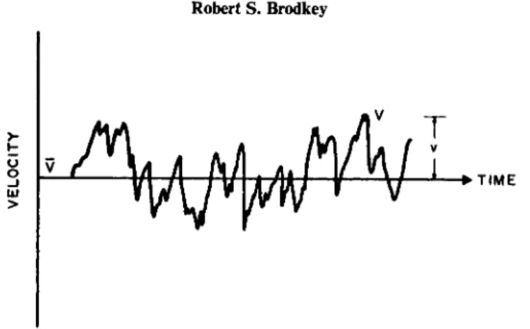
"vortex trail" in the wake of a cylinder (P3) would not be considered as turbulent motion. In other words, any motion which might have a regular periodicity is not considered to be turbulent. The instantaneous velocity ( V = i £ / + jK + kW) at a point can be represented by its average value and a superimposed fluctuation (see Fig. 1); i.e.,
U = U + u9 V = V + v, a n d W = W + w
FIG. 1. The instantaneous velocity.
where U9 V, W are the x, y9 ζ components of the instantaneous velocity, V ; 17, P, Ware the average values (a bar over symbols denotes average); and w, υ, w are the r a n d o m fluctuating components. In terms of vectors
V = V + ν
where V is the average vector velocity, and ν is the vector velocity fluctuation.
T h e vector notation offers considerable simplification in the writing of the necessary equations [for further information on vectors and vector notation seeWylie (W6)].
Certain restrictions such as isotropy and homogeneity can be impressed on the turbulent field. These restrictions, because of their simplifying nature, make the rather complex problem amenable to theoretical analysis.
The term homogeneous turbulence implies that the velocity fluctuations in the system are r a n d o m , a n d that the average turbulent characteristics are independent of the position in the fluid, i.e., invariant to axis translation.
The homogeneous system can be further restricted by assuming that in addi- tion to its homogeneous nature, the velocity fluctuations are independent of the axis of reference, i.e., invariant to axis rotation and reflection. This re- striction leads t o isotropic turbulence, which by its definition is always h o m o - geneous. T o illustrate the difference between the two types of turbulence, consider the root-mean-squared (r.m.s.) velocity fluctuations:
u = Λ / Ρ , v' = ^ / P , w' = Λ / Ρ
where w', v\ and w' are used to simplify our notation. In homogeneous turbulence, the r.m.s. values could all be different, but each must be constant over the entire turbulent field. In isotropic turbulence, the spherical symmetry requires that the fluctuations be independent of the direction of reference, or that the r.m.s. values all be equal; i.e.,
Λ / Ρ = yjv* = Λ/W* or u = ν = w'
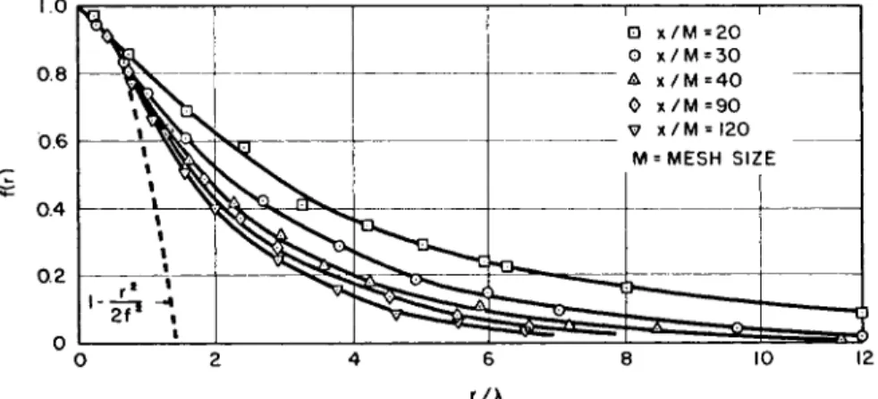
By the nature of isotropic homogeneous flow, there are no cross velocity terms (i.e., uv, uw, vw). This is a result of the r a n d o m motion which would give, for example, uv just as many positive as negative values. Consequently, the average uv would be z e r o .1 In flows of this nature then, there are no shear- ing stresses (uv is called the eddy, turbulent, or Reynolds stress, and is a part of the contribution of turbulent motion to the total shear stress τ0) and no gradients of the mean velocity. Both homogeneous and isotropic turbulence are constant space systems, and thus the statistical quantities can vary with time only ; i.e., theoretically, we would have to have a box of turbulence, which would decay with time. It is quite apparent that such a state of motion cannot be realized exactly in experiments. The grid experiments in a wind tunnel are stationary flows with decay being a function of distance from the grid rather than a time decaying system, as in theoretical homogeneous turbulence. In spite of the difference, the grid experiments can closely approximate h o m o - geneous turbulence, if one considers a small segment moving at the average stream velocity away from the grid. The segment must be small enough so that it can be considered homogeneous when compared with the inhomogeneity in the wind tunnel, but still large enough to be compared with the scale of turbu- lence (more will be said about scale shortly). For such an experiment, the decay time would be
tD = xjU (6)
and the segment would be nearly homogeneous. A thorough discussion of the problems of setting up turbulent flows for experimental study has been given by Corrsin (CI 5).
The area of turbulent study of most interest in mixing is turbulent shear flow.
This flow is the modification of completely homogeneous flow to allow for shear stresses; usually one or two of the Reynolds shearing stresses (to be discussed in more detail in Section II,B,l,g) will be zero. F o r example, in pipe flow, where u is in the direction of the pipe axis,
uw — vw = 0
and only uv is not zero and is important. Turbulent shear flow in turn may be divided into flows that are nearly homogeneous in the direction of flow, and those which are not homogeneous in the direction of flow. It has been found experimentally that the nearly homogeneous flows are those that are restricted as in pipe flow, while the inhomogeneous shear flows are unrestricted systems, such as jets. The longitudinal homogeneity (or homogeneity in the direction of flow) arises from the fact that in pipe flow, turbulence is generated and Φί(ζ)\ i-e., there is no decay. One flow of importance, which has both characteristics depending u p o n the location of study, is b o u n d a r y layer flow.
1 In contrast, u2 is always positive and thus 1? will have a value.
The area near the wall is nearly homogeneous in the direction of flow. The area near the b o u n d a r y between the b o u n d a r y layer and the ideal flow is inhomogeneous because of a n intermittent nature of the flow (Section II, These basic definitions of the types of turbulence will allow a better under- standing and further interpretation of the definitions of terms necessary to describe the p h e n o m e n a of turbulence.
b. Correlation. It was Taylor (T5) who first suggested that a statistical correlation could be applied to fluctuating velocity terms in turbulence. H e pointed out that no matter what may be m e a n t by the diameter of an eddy, a high degree of correlation will exist between the velocities at two points in space if the separation between the points is small when compared with the eddy diameter. Conversely, if the points are taken far apart, so that the space would correspond to m a n y eddy diameters, then little correlation could be expected.
Consider the velocity at two points separated by a distance r (i.e., χ and χ + r). A similarity or correlation may exist between the velocities, and can be defined as the tensor
The bar denotes an averaging, which should be taken for many points at one given t i m e ; i.e., we should have a great n u m b e r of equivalent systems. This is nearly impossible and one is generally forced to measure the fluctuations at a given point as the fluid moves relative to the measuring instrument. The Birkhoff theorem of statistical mechanics is assumed valid for turbulence.
The equivalent theorem states that if a long enough time is considered, the average at one point is the same as an average over a large number of points at one time. Thus, it is usually assumed that a time average is valid. The basis of statistical turbulence is that statistical averages can be used to describe the system. There are three components of ν at χ ; i.e., w(x), v(x), and w(x) Similarily, there are three components of ν at χ 4- r; i.e., w(x-fr), t>(x + r), and w(x + r). Consequently, if we consider all possibilities of correlation, we see that there are nine possible combinations; thus, Q(r) will have nine terms and is a second-order tensor. A n o t h e r notation (Cartesian general co- ordinates) is used more often to describe the same t e r m s ; i.e.,
where / and j can each take on three values; i.e., ι/χ(χ) = w(x), w2(x) = v(x)9
and w3(x) = w(x). As before, there are three components at χ 4- r.
A somewhat more useful correlation term is called the Eulerian correlation function, and is
B , l , j ) .
Q(r) = v(x)v(x + r) (7)
Qij(r) = wi(x)w/.(x + r) (8)
Kt( x) i/ / x+ r )
w/(x) w,'(x+r) (9)
Ui(x)Uj(x + T) ^
For isotropic homogeneous turbulence, the r.m.s. fluctuating velocities are all identical, so that Eq. (10) becomes
u 1
Further, all / φ j terms are zero, and thus the d u m m y index pair ii is used.
Batcheior (B5) has shown that only one scalar function is necessary to specify the velocity correlation. This function is generally taken as
/ ( , ) = " r W f V^ + r ) ( 1 2)
w'2
where the subscript r denotes that the velocity fluctuation is measured in the same direction as the space vector r (see Fig. 2). Another correlation, which must be related to this, is
,n( x ) » ( x+r ) u 2
where the subscript η denotes that the velocity fluctuation is measured in a direction normal to the space vector, r. As just n o t e d , / ( r ) and g(r) must be related, since only one scalar is needed to define the correlation in this totally symmetrical system. Batcheior (B5) shows, from continuity of an incompres- sible fluid, that this relation is expressed by
* / w \ ) ( 1 4
g(r) = / ( r ) + * r ( 3r
In Eqs. (12) a n d (13), the correlation functions would reduce to unity if the separation were reduced to zero. In a like manner, the functions would reduce to zero if the separation were large enough so that no correlation occurred ; i.e., just as many positive as negative values would be possible.
In the foregoing discussion, the Eulerian point of view has been taken, that is, the correlation function Ru(r) is a correlation between the instantaneous velocity fluctuations separated by a distance r. In some applications, it is more convenient to consider the Lagrangian system of coordinates, which would correlate the velocity fluctuations of a fluid particle at two times along its path ; thus
Κφ)
= "i^P,
(15)where u\ is the three r.m.s. values u\ v\ and w', which can exist and be differ- ent at χ and at χ + r. Considerable simplification is afforded if the flow is homogeneous, since the r.m.s. values will be independent of the separation.
Thus Eq. (9) becomes
where τ is some increment of time. In isotropic turbulence, the form becomes less complex; i.e.,
U *
It is very important to note that u in the Lagrangian systems is the r.m.s.
velocity fluctuation of many particles averaged along their respective fluid particle paths and not a time average at a point in space as for the Eulerian system. When the particle velocity is a stationary r a n d o m function of time, these two variances are equal. The Eulerian and Lagrangian correlations will not be the same; however, with additional information it is conceivable that they might be related. The Eulerian view is used in isotropic turbulence because fixed probes are used for velocity measurement, but the Lagrangian system is more convenient when considering turbulent diffusion and mixing because diffusion is measured by the spread of a contaminant.
The desired measurement of the Eulerian correlation is not always possible because of probe interference; however, one might assume that χ = tU is applicable and replace the space coordinate χ with an equivalent time. This in effect allows an equating of the Eulerian space correlation to a Eulerian time
correlation (autocorrelation); for example, using Eq. (12) we could say / ( r ) =^r(*)uj^) _ ur(t) ur(t + r)
u'2 u'2
F o r isotropic turbulence, this equality has been shown to be valid experi- mentally by Favre et al. (F4). For isotropic turbulence, the time correlation of Eq. (17) can be seen to be of the same form as the Lagrangian coefficient of Eq. (16). However, the time correlation part of Eq. (17) is an average of the product of the velocities taken at two times for one point, while Eq. (16) involves an average taken at two times along particle paths, and of course involves velocities along those paths. Although the autocorrelation technique can be very convenient, it is limited to cases where u is much less than U, and thus may not be valid in certain shear flows. Further discussion on this point has been given by Hinze (H5, p . 40).
When the flow is not homogeneous the shear-stress values will be finite, and a correlation will exist between the various cross velocity terms when the separation is zero or finite. F o r zero separation, Eq. (9) will reduce to a point correlation which is
Ru = ^ (18)
U,Uj
The functional dependence on χ is usually dropped from the notation, since all terms are understood to apply to a single point; however, this does not mean that the correlation will not vary from point to point. In the point correlation, if / = j \ the function is trivial and is always equal to unity.
Other higher order velocity correlations are possible. F o r example, the triple velocity correlation appears in conjunction with the double velocity correlation in the Kârmân-Howarth equation (to be discussed in Section II,B,l,g). The form of the triple velocity correlations is analogous to Eq. (8)
Sijk(r) = n,(x) uj(x) uk(x + r) (19)
This correlation can have 27 terms and is a third-order tensor. Batcheior (B5) points out that as in the double correlation, the important velocity fluctuations that are measured are either in the same direction or normal to the position vector r.
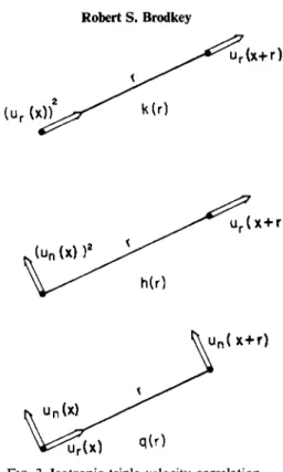
For isotropic turbulence (see Fig. 3) there are three different correlations which are expressed as
k(r) = " Λ * )2 " r(x+ r )
m
- ^ i O ^ t l ) (20)
q(r) = "Λ*) un(x) un(x + r)
FIG. 3. Isotropic triple velocity correlation.
It should be added that the first of these is the easiest to measure, since it involves only velocity fluctuations in one direction. The other two are related to this one, because only one scalar is necessary to specify the triple velocity correlation in isotropic turbulence.
In turbulent shear flow, there exists a triple velocity correlation at a single point, just as there exists a double velocity correlation at a single point [Eq. (18)]. These triple correlations have been measured in a few flows;
however, the experimental errors are so large that the results have only quali- tative value.
c. Intensity. The intensity of turbulence is defined as the r.m.s. values of the fluctuating velocities; i.e.,
u' =
V ?
V =
y/W
(21)The intensity, r.m.s. value or variance is sometimes expressed as a fraction or percentage of the mean flow velocity; i.e., for example u'jU.
d. Scale. The scale, which is sometimes pictured as the average size of the eddies, has several possible definitions depending upon the choice of the cor-
relation function. If one first considers the Eulerian system of coordinates, a scale can be defined as the area under the correlation versus separation curve [Rij(v) vs. r], i.e.,
L = j X ( r ) c / r (22) F o r isotropic turbulence (Batcheior, B5) the longitudinal integral scale (r) is
defined as
00
Lf = jf(r)dr (23)
0
and the lateral integral scale (n) is defined as
= \g(r)dr (24) g
ο
This scale is also called the "transverse Eulerian scale," i.e., the separation vector is taken normal to the direction of flow. S i n c e / ( r ) and g(r) are related as shown in Eq. (14) there must be a relation between the scales; this relation
Lg = \Lt (25)
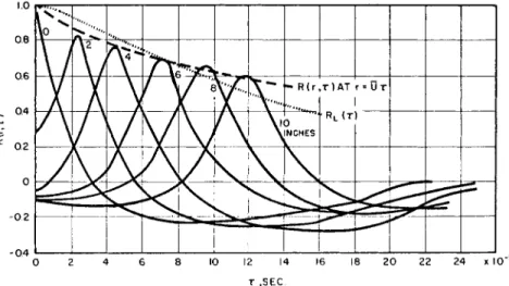
The notation /2 or Ln is sometimes used for the Eulerian scale, Lg, and /0 for Lf. The Lagrangian coordinate system follows the path of a particle, and the correlation is given by Eq. (16). Although this system of coordinates is much easier to use in many cases, measurement of the corresponding correlation, Rl(T), is complicated. Recently, Rl(T) has been estimated from turbulent diffusion measurements in turbulent shear flow [Baldwin (Bl)] and for a decaying isotropic turbulence in the wake of a grid in a wind tunnel (Uberoi and Corrsin, U l ) . A time scale based on the Lagrangian coordinate system would be
Tr = \ = JRLij(r)dr (26)
Several Lagrangian length scales can be defined; the transverse Lagrangian scale is defined as
LL = v'TL (27)
Another Lagrangian length scale is defined as
AL = VTL (28)
The ll9 is sometimes used for LL by some authors.
T h e relation between the Lagrangian and Eulerian scales has not been established from theory; the scales will vary in many cases by some numerical value that will be dependent on the nature of the fluid motion and will have to be determined by experiments. F o r now, it will suffice to point out that the
ratio of LLjLf has been reported as varying from 2 to 6.5 for various condi- tions. Further comments on the relation of the Eulerian and Lagrangian systems will be made during the discussion of turbulent diffusion, since this LJLf ratio is essential to obtaining values in the Lagrangian system.
e. Spectrum. The equations descriptive of the turbulent velocity field involve the double and triple velocity correlations [Eq. (46)]. A considerable simpli- fication can be made if the Fourier transform of the equation is used [Eq.
(47)]. The Fourier transform is simply the means by which the complex random wave form of the turbulent motion can be broken into a sum of sine waves of various amplitudes and frequencies. The sum of the sine waves must equal the original wave form. In general, the spectrum is reported as a plot of the amplitude of the various sine waves against their respective frequencies. The analysis involves taking the transform of the various correlations already considered. The transformed correlations are of the form of an energy spectrum and can provide insight into the distribution of the kinetic energy of turbulence over the frequencies of the velocity fluctuations (frequency can be pictured roughly as an inverse eddy size).
This important mathematical advance was made by Taylor (T6); he con- sidered only the one-dimensional spectrum, but Heisenberg (H4) and others have expanded the analysis to the three-dimensional space spectrum. The Taylor theory showed that by an application of the theory of Fourier trans- formation to a statistically steady field [as defined by the correlation Qyir) in Eq .(8)] one could arrive-at the Fourier transform of the velocity correlation tensor, or the energy spectrum tensor. In mathematical terms of a Fourier transformation, and in tensor notation, the spectrum is
where / in the exponent is y/ — 1, and k is the wave number vector. The com- ponents of this vector are related to the frequency (ή) by
In effect we have broken down a complex wave (in real space x) into a number of sine waves (in frequency space). Generally, this frequency space is referred to as wave number space (k), where the wave number is related to the frequency (29)
kt = InnJUi (30)
by Eq. (30).
For the reverse transformation,
oo
(31) The term dk is understood to mean
dk = dkt dkj dkt
In other words, it is an element of volume in wave number space about the vector k.
If r = 0, then this reduces to
00
ββ( 0 ) = / Φ( , 0 0 Λ ( 3 2 )
- 0 0
where Q,j(0) is the energy tensor. T h e energy spectrum tensor, <£,7(k) can be pictured as being an energy density in wave number space. By analogy to mass, the a m o u n t is equal to the total integral over the volume of the point densities times the differential volume. In the analogy, k is the volume, dk the differen- tial volume, ^,/(k) the density, and β,7(0) the mass.
It has already been indicated that the triple velocity correlation will appear in the equations of motion when they are in terms of the correlation functions.
T o solve these equations, they are reduced by Fourier transformations to simpler differential equations. It is therefore necessary to introduce the triple velocity correlation Fourier transformation; this is given by
00
W i J k { k) =
( 2 π ? jsijk(T)e-ik-'dr ( 3 3 )
- 0 0
where ^ . ( r ) was given in Eq. (19). Its transformation is
00
SuJr) = J Wuk(ky*'dk ( 3 4 )
- 0 0
Both the Kârmân-Howarth equation and its Fourier transform, which contains the various spectra terms, will be presented in Section II,B,l,g.
The spectrum tensor is the transformation of the correlation tensor from Eulerian space to wave number space, and it can be pictured as a tensor that describes how the energy, associated with each velocity component, is distrib- uted over various wave numbers of frequencies. In essence, a Fourier analysis of the complex turbulent fluctuations will give a spectrum of the turbulent energy associated with a given wave number or frequency. The wave number is often considered to be a measure of the reciprocal of the eddy sizes; however, this should not be taken literally and interpreted as specific eddies of a given size actually rotating in the fluid.
The spectrum tensor is quite complicated and cannot be measured completely. The one-dimensional spectrum function proposed by Taylor can be measured by an electronic harmonic analyzer operating on the output of a turbulence detector, such as a hot-wire unit. This one-dimensional spectrum function is defined as the integration of the energy spectrum tensor over all possible lateral values of k :
00 00
M*,) = j J0u(k)dkjk„ (35)
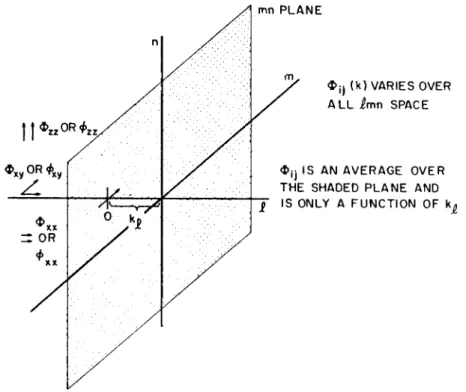
The subscripts Imn are used to denote components just as are ijk, but the two sets may operate separately. As shown in Fig. 4, the one-dimensional spectrum is a summation of ^/ 7( k ) over a plane (mn), which is located at a distance kl
from the origin (k). Thus this spectrum, Φ^ι), must depend on kl. The actual measurements, for example, for pipe flow, might be the one-dimensional spectra associated with the three intensities of Eq. (21) and the one possible shear term discussed in Section II,B,l,a. To make the analysis, these various instantaneous signals would be fed into a spectrum analyzing apparatus.
FIG. 4. The one-dimensional spectrum function.
A modified tensor can be obtained by integrating the energy-spectrum tensor over wave number space, k. The integration is performed over a spheri- cal surface of radius, k = | k | ; the resulting term is called the integrated energy spectrum tensor:
Eu{k) = J0o(k)dS(k) (36)
In this equation, dS(k) is an element on the surface of the sphere of radius, k.
Since E^k) is a product of a density and an area term in wave number space, it can be pictured as the energy contribution per wave number. Thus El}(k)dk would be the contribution to the energy tensor, £?/,(()), from wave numbers in
u K ' w/(x) Uj(x + r)
(3) Eulerian correlation function for isotropic turbulence:
/ ( r ) = r (Mx) " r ( * + r) (1 2)
g ( r) =. «„(*) «,,(* + •·) ( Β )
(4) Lagrangian correlation function :
RL.{r) = ^UJ!±U ( 1 5 )
the range of k to k 4- dk, which is the space between spheres of radii k and A: + dk in wave number space.
Another term associated with spectrum is the three-dimensional energy spectrum function, which is defined as
E(k) = *£„(*) (37) This term is the kinetic energy density per wave number. T h e total kinetic
energy is the integration of this over all wave n u m b e r s ; this, then, is
00
ÏQM = \7f = i(I? + P + P ) = JE(k)dk (38)
0
The foregoing spectral equations are greatly simplified by the assumption of isotropic homogeneous turbulence, for, as has been seen, the correlation tensor could be represented by a single scalar, and so it must be with the spectrum tensor. In addition, a number of interrelations can be derived for the terms so far defined. All of these are covered in detail in Chapter III of Batchelor's book (B5).
For isotropic turbulence and for a sphere of radius k in wave number space (area = 4t t / c2) , Eq. (36) can be integrated directly to give
E(k) = \Etffc) = 4 ^ ( i ) 0 , ( k ) (39) Identical subscripts are used since the ij terms do not exist in isotropic
turbulence. Generally, E(k) is used as the single scalar function describing the energy spectrum tensor.
/. Summary of Terms. In the preceding sections the following terms have been discussed.
(1) Eulerian correlation tensor:
Ô,y(r) = M (.(x)W,(x + r) (8)
(2) Eulerian correlation function :
(5) Lagrangian correlation function for isotropic turbulence:
R = u(t)u(t + r)
L u'2
(6) Eulerian triple correlation function for isotropic turbulence :
h(r) = Κπ (χ)8" γ (Χ + Γ )
= ur(x)un(x)un(x + r)
(7) Intensity:
u'
= Vw
2,
v' = \/v2 , w' = \Jw2 (8) Eulerian scales:oo
Lf = jf(r)dr
Lg = jg(r)dr
0
( 9 ) Lagrangian scales:
oo
TL = JRLifr)dr
0
LL = v'TL
( 10) Energy spectrum tensor :
00
- 0 0
(11) Energy tensor:
00
Q,i(0) =
J *<W <*k
( 1 6 )
( 2 0 )
( 2 1 )
( 2 2 )
( 2 3 )
( 2 4 )
( 2 5 )
( 2 6 )
( 2 7 )
( 2 9 )
( 3 2 )
(12) One-dimensional spectrum function :
OO 00
<£,#;) = j faiVdkJK (35)
- 0 0 - 00
(13) Integrated spectrum function :
E,j(k) = j 0u(k)dS(k) (36)
(14) Energy spectrum function :
E(k) = \Eu{k) (37)
g. The Equations of Turbulent Motion. In the following paragraphs, it is shown how the fluctuations which occur in turbulent flow result in added terms in the basic equations of laminar motion. If an exact representation of these fluctuations were known, a general solution might be obtained to account for turbulence. The nature of the additional terms was first investi- gated by Reynolds (R4). He assumed that the point velocities in the laminar flow equations could be replaced by the instantaneous point velocities in turbulent motion, and that the equations would still be completely valid.
Thus, he combined the Navier-Stokes equations for laminar motion with the concept of an average velocity and a superimposed fluctuating component.
He then averaged the resulting equation and used certain rules of approxima- tion, which he formulated, to allow calculation of mean values. These rules are not rigorous, but are good approximations when the fluctuations are sufficiently numerous and are distributed at random.
Reynolds found that for incompressible flow, the equation of continuity was identical, except that the instantaneous velocity was now replaced by the average value at that point; i.e.,
_ + _ + _ = 0 or -τ-1 = Ο (40)
οχ oy cz ύΧι
οχ dy οζ οχ{
The equations on the right use the general Cartesian notation, in which a repeated index implies summation over its three values. This is sometimes written
For the Navier-Stokes equations, he found that again average properties appeared in place of point properties and that an additional term was added, which is associated with the fluctuations. For comparison, the two equations are:
26
Navier-Stokes
[ dt
Jd
XjJ
dx; dxfix:Reynolds
p\dt J
8xjJ
dx, ^dxjBxj ' eXiv '
For the benefit of the reader not familar with the notation, Eq. (43) for ι = 1 is
pi— + Ό— + F — 4- W—\ = - ^ + μ(— + — +
^z2 /
- &
+ί?
+Ψ)
(44)the repeated index in any one term is j9 and summation is made over its three values. There are two additional equations possible; i = 2 and / = 3. The notation of Eq. (43) saves considerable writing, since only one general equa- tion need be used.
The additional term has nine components, three of which are shown for the x-equation [Eq. (44)]. The term pujUj is called the eddy, Reynolds, or turbulent stress. The tensor in Cartesian coordinates is
(
w^ uv uw\ vu ν2 vw\ (45)wu wv w2/
The tensor is symmetrical, since uv = vu, uw = wu, and vw = wv. Thus there are only six independent terms.
The Reynolds equations for incompressible turbulent motion cannot be solved, for there are ten unknowns and only four equations available: the three motion equations and one continuity equation. The unknowns are the mean pressure, three average velocity components, and six Reynolds stresses.
Karman and Howarth (K4) investigated the incompressible Navier-Stokes equations at two points, separated by a distance r in a homogeneous turbulent field. This study at two different points introduces the concepts of correlation.
They obtained an equation which involves double and triple correlations and correlations between the pressure and velocity fluctuations. The entire equation can be transformed into terms of the spectrum tensors. Considerable simplification can be effected if isotropic turbulence is assumed. For example, the velocity field is uniform, so that the lateral (//) pressure terms must be zero. In isotropic turbulence, the only concern is with the inertial terms, which provide the transfer of energy between the different eddy sizes or wave numbers. Since the various tensors can be reduced to scalar functions, the
27 tensor equation reduces to a scalar equation under the restriction of isotropic turbulence. In terms of correlation,
This is the Karma n-Howarth equation for isotropic turbulence, in which all the terms can be obtained experimentally; Stewart (SI2) has found that the equation is correct within the experimental error of his measurements.
The isotropic equation in terms of spectrum is
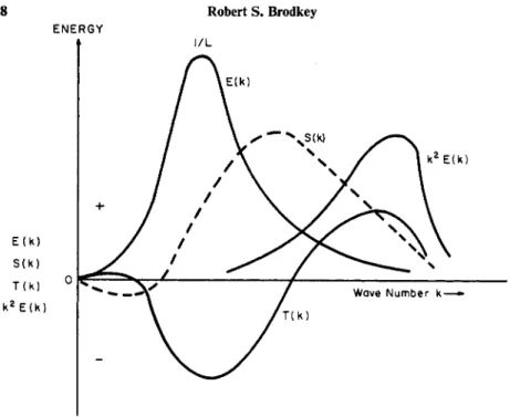
8I^} = T(k) - 2vk*E(k) (47)
where E{k) is defined in Eq. (37), and T(k) is the corresponding transform of a triple velocity correlation. The scalar T(k) is associated with the transfer of energy between wave numbers or eddy sizes. Townsend defines a transfer function
k
S(k) = - JT(k)dk (48) ο
which is the total energy transferred from eddies in the range of 0 to k, to those in the range greater than k. Using this modification, Eq. (47) becomes
i E { k) = - 8 ψ - 2,-k*W) (49)
dt ok
Equations (47) and (49) show that the viscous dissipation reduces the energy from components of any one wave number, but has no effect on the transfer between wave numbers. Further, this energy dissipation is selective toward the high wave numbers or small eddies, because of the strong effect of the k2 factor. If continuous decay is assumed, so that dE(k)jdt is always negative, then S(k) must always be positive and displaced toward the low wave numbers or large eddies, for the energy must be transferred from these large eddies to the smaller ones where it will be dissipated by viscous forces. A picture of these scalar functions is given in Fig. 5. The transfer function T(k), is of the form suggested by Proudman and Reid (P6) and Kraichnan (K17). By using Eq.
(48), S(k) was obtained by integration.
Actually, Eqs. (46) and (47) cannot be solved since in each case there are two unknowns and only one equation. A new equation for the triple velocity correlation can be constructed in a manner analogous to that just done for the double velocity correlation. However, due to the nonlinearity, in this new equation, inertial terms of the fourth order appear, and if one were to write the fourth-order equation, the terms for the fifth order appear. This constitutes one of the major problems of turbulence, for although any number of equations can be generated, there is always one more unknown than equations.
FIG. 5. The scalar functions for isotropic turbulence.
This infinite hierarchy of dynamical equations gives rise to what is called
"the closure problem of turbulence theory." The problem is: by what means can we replace the indeterminate infinite set by a plausible determinate finite set, and thus gain some useful information about turbulence?
A considerable segment of the work on turbulence has consisted of attempts to obtain solutions or approximations to these equations. The form and time dependence oÎE(k), the energy spectrum function, has been diligently sought.
Some of these efforts will be indicated here; however, no details will be given.
It should be strongly emphasized once again that the description of turbulent mixing in a turbulent field always includes the unknowns from turbulent motion, which must be understood before one can successfully solve the turbulent mixing problem.
h. Solutions of the Equations of Turbulent Motion. In order to obtain a solution to Eq. (47), some assumption or development must be made to obtain a relation between E(k) and T(k). One possible method is to assume that the decay process is independent of T(k); thus, the inertial effects can be assumed to be negligible. Batcheior has analyzed the problem of very low wave numbers or the very large eddies; in essence, his argument can be seen from Fig. 5.
The inertial or transfer term, S(k), and the viscous term, k2E(k), fall off more rapidly than does the spectrum function, E(k), as k 0. From this one can conclude that the big eddies have little interaction with the remainder of the
ENERGY
t
l / L_ ο - EQU/
- EQU/
·· CONv APPF DAT/!
VTI0N(5 moN(«
IECTUR Î0XIMA 2) 51) FINA ED FOR TION
L PERI HIGHEF
OD X ORDE R
Ô
turbulence, and thus change very little during the process of decay. In other words, in the vicinity of k = 0, the spectrum function does not change. Near the end of the decay period, the energy in the smaller eddies will have been dissipated, and at some point in time the controlling factor will be the supply of energy from the very large persistent eddies to viscous dissipation. When only the large eddies remain, the energy is concentrated toward the low wave numbers and the inertial term is negligible. Thus, by setting the inertial term to zero, the final period of decay is considered. This assumption leads to the result that near k = 0, E(k) varies as A;4, and that E(k,t) decays as follows:
E(k,t) = E(k9t0)e-2vk2{tto) (50)
Combining this with Eq. (38) gives the decay in intensity:
Û2 = 2A[v(t-t0)Y5A (51)
The agreement with the experimental data is excellent. For example, Fig. 6 shows a curve computed from Eq. (51) and the experimental data of Batcheior
240 200
160 Ν
fo 120 60 40
0
- 4 0 0 -200 0 200 400 600 800 1000 x/M
FIG. 6. The final period of decay [by permission from Deissler, R . G., Phys. Fluids 1, 111 (1958)].
and Townsend (B8) for flow in a pipe downstream of a grid or screen. In Fig.
6, M is the grid or screen opening, χ is distance downstream from this screen, T? is the mean-square velocity fluctuation and U2 is the average fluid velocity squared. Distance, x, in Fig. 6 is related to time, t, in Eqs. (50) and (51) by the relation, χ = Dt. This figure is from a recent article by Deissler (D5), in which he derived an equation for the triple correlation. In his final equation to be solved, he neglected the inertial terms of the fourth order, which are analogous to T(k) in the two-point equations ; this has been called the higher-
order moment, discard approximation for closure. The equation, when solved, was
? = 2 Λ Κ ί - ί α ) ] - Κ + 2(B/v)
Κ^ίο)]"
7 (52)The constants A and Β are determined from the initial conditions. As can be seen from Fig. 6, Eq. (52) represents the decay for times considerably before, as well as during, the final period of decay. Deissler (D6) carried this approach to the fourth-order equation, and neglected the inertial terms of the fifth order. He obtained improved agreement ; however, he pointed out that mathe- matical complexity would prevent this procedure from being carried out ad infinitum.
Another approach is to find a nonzero relation between E(k) and T(k) and not to restrict oneself to the final period by neglecting the higher order inertial terms. This approach has involved some kind of heuristic argument to establish the desired relation. In effect, this is a limited model approach, where a mechanism is suggested for the energy transfer; this method is generally called the phenomenological approximation for closure. Karman (K19) has suggested the form
oo k
S(k) = c\k'y[E(k')Y dk' Jk^^EnM^dk" (53)
k 0
where C is greater than zero, and β and γ are constants. This form includes the Heisenberg (H4) suggestion, where C = 2α, β = 1/2 and γ = - 3 / 2 . Equation (53) can be thought of as a mathematical representation of the hypothesis that energy transfer between eddies occurs by a stress-strain mechanism, where the strain is provided by the large eddies, and the resistance to strain or the stress by the small eddies. Tanenbaum and Mintzer (Tl) have used the data of Stewart and Townsend (SI3) and Stewart (SI2) to establish empirically the best values of α, β, and γ, They suggest 0.60, 1/4, and —5/2 respectively;
however, good results were obtained for 1 /2 > β > 0, and — 3/2 > γ > — 7/2.
A more recent argument has been put forward by Batcheior et al. (B7). In the discussion on turbulent mixing, we will have occasion to refer back to Eq.
(53). For the details of the many ramifications of Eq. (53), the reader is referred to the book by Hinze (H5).
The next logical step from the mathematical standpoint is to relate the highest order moment to lower order moments present in the system of equations; in other words, to postulate some statistical assumption for the joint probability distribution of the turbulent field. Millionschtchikov (M6) was the first to introduce the quasi-normal joint probability distribution between the second- and fourth-order moments. The potential simplicity of the method lead Proudman and Reid (P6) and Tatsumi (T2, T3) to use the approximation for studying the dynamical behavior of turbulent motion.
Their results are valid only for short periods of time after the initial specifica-
31 tion of the turbulence spectrum. Ogura ( 0 3 , 0 4 , 0 5 ) has shown that for long times the approximation leads to unreal results; i.e., a part of the spectrum decays so fast that it becomes negative, a physical impossibility. O'Brien and Francis ( 0 2 ) and Kraichnan (K15) have shown that a similar phenomenon occurs when a scalar field in turbulent motion (mixing) is considered.
Unfortunately, most of our interest is in flows where the Reynolds number is high and the approximation fails.
From a theoretical standpoint, the previously discussed closure methods leave much to be desired. More complex approximations have been suggested, but for the most part they are so complex that actual solution seems unlikely.
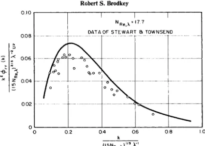
One exception to this is the stochastic model approximation presented by Kraichnan (K12-K17). The first approximation for isotropic turbulence is called the "direct-interaction model" and treats the third order transfer term in an equation similar to Eq. (49). This term involves the distribution of energy across k, but involves no net change. The major advantage of the approach is that the resulting equations describe a model which replaces the real problem. This model is described without approximation, and as a result unreal effects such as a negative spectrum should be avoided. The degree of approximation to the real problem must be established by asking how closely the model represents true turbulence measured by experiments. The solution is by no means easy and has only recently been accomplished by a direct- numerical integration method. At moderate Reynolds numbers, a reasonable description, free of inconsistencies, was obtained (K17). At high Reynolds numbers the general numerical accuracy was poor. As an example of the reasonableness of the computation, Fig. 7 compares the experimental data for the one-dimensional dissipation spectrum k2<f>rr(k9t), with calculated results.
For higher Reynolds numbers, a higher order approximation may be needed.
Finally, it should be noted that the direct-interaction model can be generalized so that it is not restricted to isotropic turbulence (K16). However, even in its simplest form, it may find application to those shear flows for which the actual turbulence level is not too great (K17).
Much of the work in statistical turbulence has investigated the system, Eq. (47) and higher order equations, under certain limiting conditions. The study of the final period of decay, already discussed, is representative of these studies. Another well-known approximation is that of local isotropic turbu- lence, in which an intuitive model is introduced.
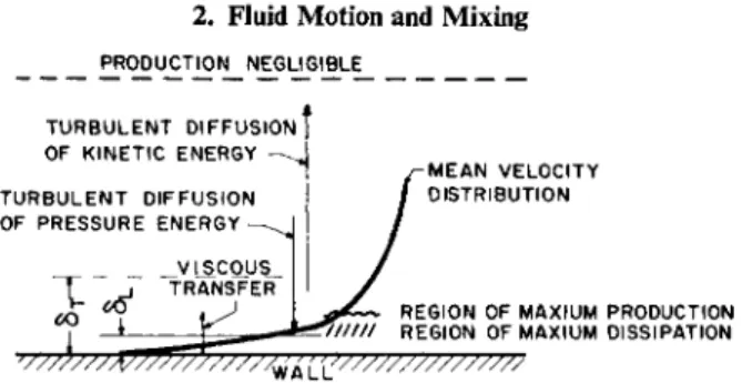
Consider flow in a pipe at some relatively high Reynolds number. Through- out the pipe, the viscous forces along the wall provide the conditions necessary for turbulence formation; very large vortices, or large eddies, arise from the interaction of the mean flow with the boundary. The scale of these large eddies would be comparable to the size of the system or, rather, to the distance over which the mean flow velocity changes. In pipe flow, this size would be of the order of the pipe diameter.
32
ο.ιο
0.08
0.06
2 0.04
0 0 2 h
ο
ι 1 I I I I0 0.2 0.4 0.6 0.8 1.0
k
FIG. 7. The one-dimensional dissipation spectrum [by permission from Kraichnan, R. H.
Phys. Fluids 7, 1030 (1964)].
The inertial forces in the system give rise to the transfer term S(k), which is a measure of the transfer of energy from the larger eddies to the smaller ones.
In other words, the motion of the large eddies is unstable and will give rise to smaller eddies of an order of magnitude smaller. These smaller eddies in turn are unstable and give rise to still smaller eddies; this process continues until eddies of the smallest size are formed. The mechanism of the transfer is not stated, and in fact is not needed at this point; however, it might be a breakup of the large eddies or a creation of new smaller eddies by some inertial stress- strain interaction. For all but the smallest eddies, the Reynolds number (based on the eddy size) is large, and dissipation by viscous forces is unimpor- tant. As the eddy size decreases (wave number increasing), the Reynolds number becomes smaller and smaller, and at some critical point viscous forces become important. The suggested model is a cascade of energy from the large to pro- gressively smaller eddies, until it is lost to heat by the dissipation action associated with the smallest of eddies. Viscosity is associated with the two extreme ends of the process ; it is both the creator and destroyer of the turbu- lence, but does not have any net effect in the middle range of energy exchange.
One may imagine that as a consequence of this mechanism, the boundary affects the largest eddies the most strongly (creates them) and loses its effect as the process moves down the chain of eddies. At the very high wave numbers or small eddies, the effect of the boundaries is completely lost or is negligible.
Thus the small eddies can be visualized as being independent of the boundaries or mean flow.
In the nonhomogeneous system, pressure forces are expected to exist and would act in the direction to make the flow isotropic. One can now assume that
33 the motion for the small eddies is isotropic because of the tendency created by the pressure forces and the independence of the small eddy motion from the boundaries and mean flow. This assumption leads to the conclusion that there is a range of wave numbers associated with the small eddies which is stationary or statistically steady, responsible for the viscous dissipation, and not directly dependent on the energy-containing eddies; that is, the very smallest eddies must be in a state of equilibrium. The only terms upon which this equilibrium state can depend are the rate of energy input and the dissipa- tion of energy. Further, if these eddies are in balance, then the rate of energy input must equal the dissipation rate. This theory, first postulated by Kolmogoroff (K8-K10), states that the eddies in this equilibrium state will depend only on the rate of energy dissipation or input, ε, and on the kinematic viscosity, v. The kinematic viscosity will determine the rate at which kinetic energy can be dissipated into heat. This theory is known by several names:
local isotropic turbulence, local similarity, and universal equilibrium.
The system of turbulence of this hypothesis can be pictured in terms of the energy spectrum of Fig. 5. The term E(k), the energy-containing eddies, is distributed toward the large eddy sizes; this energy is transferred by the term S(k) toward the smaller eddies where the dissipation k2E(k), takes place. If the small eddies are considered to be in equilibrium, then the controlling factors are ε and v. Dimensional analysis can be used to find the necessary form for a length and velocity parameter to characterize the equilibrium area. The dimensions of ε and ν are
The length η can be considered as an internal scale of local turbulence for the equilibrium range, as contrasted with an external or integral scale, L, of Eq. (22), which would be descriptive of the over-all turbulent motion. The scale, L, is a measure of the velocity fluctuations which can cause a hot-wire unit to react, and thus is a measure of the eddies which contain the turbulent energy. To an order of magnitude approximation, L can be taken as the point of the maximum in E(k), the energy-containing group. In a like manner, η is associated with the viscous dissipation group, and can be taken as the point at which the maximum in k2E(k) occurs (see Fig. 5).
For the equilibrium range to exist, the energy input by transfer, S(k) = ε, must equal the energy dissipated by kinematic viscosity; this balance can be shown as
e(L2T~*) viL2^1) The combinations for a length and velocity parameter are
(54)
00
(55)
0
Comparison with Eq. (49) shows that the term dE(k)jdt must be negligible.
The equilibrium range of eddies can depend to some extent on the structure of the large energy-containing eddies, but must be independent of the time rate of decay of the turbulence. It is hard to see how this would be possible unless η <^L9 that is, the energy-containing eddies are separated in size from the equilibrium dissipation range of eddies. If the separation is large, that is, if the viscous dissipation eddies are entirely in the equilibrium area, Townsend (T16) has determined from his experimental work that the centroid of the equilibrium range (balance point) is near Ο.5/77. From Fig. 5, one can see that η is also a good measure of the smallest energy-containing eddy. Thus the smallest detectable energy-containing eddy or turbulent fluctuation will be of the order of η ; i.e.,
smallest turbulent eddy = νΛεν* (56)
From dimensional analysis, the form of the spectrum E(k) over an equilibrium range must be
E(k9t) = ν2ηΨψη) (57)
where Ψ$η) is a universal function. Combining Eqs. (53) and (57) gives
E(k,t) = v5/*eiAW(kv) (58)
If the Reynolds number were high, so that it would be possible for some of the larger eddies in the equilibrium range to be independent of viscous dis- sipation, then for these eddies, the inertial term S(k) will be most important.
This state is called the "inertial subrange." The eddies in this range are still small enough to be independent of the boundaries and to remain in the equi- librium range. However, they would be too large to dissipate energy directly by viscous forces. Thus, these eddies receive energy from the larger ones and then transmit this energy to the small dissipative eddies. Batcheior has shown that the required Reynolds number for the inertial subrange is about twice that required for the equilibrium range to exist. However, if such a range could be realized, then Ψ$η) must be of such a form as to make Eq. (57) or Eq. (58) independent of the kinematic viscosity. The form would be (£77)"^, and Eq. (58) would become
E(k9i) = νΑεΧΛΑ\νΛ\ελΛγΛ^Λ = ΑεΛ^Λ (59) where A is a constant.
In contrast to Eq. (59), Kraichnan obtains E(k9t) = constant (ew')HAr^
which is small in terms of the difference in k(ky«)9 but important in the addi- tional term u'9 the r.m.s. velocity. The implication is that the inertial range is strongly dependent on the energy-containing range of eddies. However, Kraichnan (K22) has shown that the —3/2 range is a result of inadequacies
![FIG. 6. The final period of decay [by permission from Deissler, R . G., Phys. Fluids 1, 111 (1958)]](https://thumb-eu.123doks.com/thumbv2/9dokorg/1156570.83593/23.648.153.500.397.680/fig-final-period-decay-permission-deissler-phys-fluids.webp)