1 Int. J. Global Warming, Vol. 18, No. 1, 2019
1
A framework for predicting the effects of climate change on the annual
2
distribution of Lyme borreliosis incidences
3
Ákos Bede-Fazekas*
4
Institute of Ecology and Botany, 5
MTA Centre for Ecological Research, 6
Alkotmány u. 2-4., 7
H-2163 Vácrátót, Hungary 8
and 9
GINOP Sustainable Ecosystems Group, 10
MTA Centre for Ecological Research 11
Klebelsberg Kuno u. 3., 12
H-8237 Tihany, Hungary 13
Email: bede-fazekas.akos@okologia.mta.hu 14
*Corresponding author 15
16
Attila J. Trájer 17
Department of Limnology, 18
University of Pannonia, 19
Egyetem u. 10., 20
H-8200 Veszprém, Hungary, 21
Email: attila.trajer@mk.uni-pannon.hu 22
Abstract: Global climate change is predicted to affect both the spatial and annual 23
distributions of vector-borne diseases. Tick-borne diseases are particularly sensitive to 24
the changing climatic conditions. Modeling them is, however, challenging due to the 25
input-intensity of these models. A framework with low number of inputs (easily 26
accessible weekly temperature data and week numbers) on modeling the seasonality of 27
Lyme borreliosis incidences is presented. The modelling framework enables predicting 28
the annual distribution of Ixodes ricinus tick's biting activity and Lyme borreliosis in 29
two cascading phases, incorporating a population dynamics approach. The model is 30
calibrated for Hungary as a case study, for the period of 1998–2008, using tick-borne 31
encephalitis series as a proxy for biting activity. Prediction to the future period of 2081–
32
2100 is also provided. Climate change may significantly alter both the annual 33
distribution of I. ricinus activity and that of the Lyme borreliosis incidences. The 34
currently unimodal annual distribution of Lyme borreliosis is predicted to become 35
bimodal with a long summer pause and a spring maximum shifted 8 weeks earlier.
36 37
Keywords: Lyme borreliosis; climate change; Ixodes ricinus; tick-borne encephalitis;
38
prediction 39
40
Biographical notes: Ákos Bede-Fazekas is MSc in landscape architecture, BSc in 41
software development, PhD in agricultural engineering sciences, and research fellow at 42
Hungarian Academy of Sciences (MTA). His main research interest is in predictive 43
ecological modeling in R statistical software and the impact of climate change.
44 45
2 Attila J. Trájer is doctor of medicine (MD), PhD in health sciences, PhD student of the 46
Doctoral School of Chemistry and Environmental Science of University of Pannonia 47
and research fellow at University of Pannonia, Veszprém, Hungary. His main field of 48
research is the impact of climate change on vector-borne diseases and the ecology of 49
arthropod vectors.
50 51
3 1.INTRODUCTION
52
The anthropogenic climate change, a gradual, long-term alteration of worldwide 53
weather patterns caused by the increasing concentration of greenhouse gases (Jaha and 54
Ekumah 2015; Zhong 2016; Aleixandre-Tudó et al. 2019), influences the complex 55
society-biosphere-climate-economy-energy system (Akhtar et al. 2019), including 56
diseases and their prevalence (Ofulla et al. 2016). Climate affects the human behaviors 57
and activities, the structure of the settlements, the population of the host and reservoir 58
mammals, the conditions of the potential tick habitats, and therefore, these mankind- 59
induced effects change the pathogen transmission and, finally, the incidence of human 60
tick-borne diseases (Lindgren 1998). Tick-borne diseases are the products of a complex 61
chain of environmental factors (Epstein 1999). Changing climatic and other 62
environmental factors affect the seasonality of the acquiring of tick-borne diseases via 63
the alteration of the daily, the inter-annual and the long-term patterns in risk of infected 64
tick bites (Lindgren and Jaenson 2006).
65
Ticks are small ectoparasite arachnid arthropods living by feeding on the blood 66
of different homoiotherm and poikilotherm tetrapods. More than two dozen tick species 67
occur in Hungary, but the sheep tick (Ixodes ricinus L. (Acari: Ixodidae)) is the most 68
important in the aspect of environmental health. I. ricinus is the most common vector of 69
Lyme borreliosis and also one of the most common ticks in many parts of Europe 70
(Földvári and Farkas 2005; Rizzoli et al. 2014). The observed temporal and spatial 71
expansion of the species in the past decades has been correlated to changes in climate of 72
Europe (Lindgren and Jaenson 2006). It was concluded by several authors that climate 73
change will lengthen the vegetation season and, consequently, the activity period of the 74
different vector species (Hunter 2003; Rogers and Randolph 2006).
75
In the aspect of the adaptation strategies of medical and personal practices (i.e.
76
the seasonal use of tick repellents, vaccines, the behavioral avoidance strategies) the 77
distribution (i.e. seasonality, length and the peak) of the incidence of tick-borne diseases 78
is more important than the total yearly incidence of them. In Hungary, the questing 79
activity of I. ricinus nymphs and adults starts in March, reaches its maximum in April, 80
shows its summer minimum in August and its second, less expressed peak in October 81
(Széll et al. 2006; Egyed et al. 2012; Trájer and Földvári unpublished data). Despite of 82
the bimodal distribution of tick activity and tick-borne encephalitis the distribution of 83
Lyme borreliosis is unimodal (Zöldi et al. 2013; Trájer et al. 2014). Gray (2008) 84
forewarns that the annual distribution of both I. ricinus activity and Lyme borreliosis 85
may change significantly in the future due to climate change. It is therefore required to 86
investigate the impact of climate change on their annual distribution (Ogden et al.
87
2005).
88
The development and activity of I. ricinus ticks, and the number of the questing 89
ticks are related to the seasonal variation of temperature, in addition to that of other 90
abiotic factors (e.g. humidity and photoperiodicity) that are hard to access or 91
incorporate in a model (Randolph 2009; Jore et al. 2014; Cat et al. 2017). The 92
relationship between temperature and both the interstadial development rates and the 93
daily questing rate is non-linear (Randolph 2004; Trájer et al. 2014).
94
The aim of our study is to (1) build a framework with low number of inputs on 95
modeling the annual distribution (seasonality) of Lyme borreliosis incidences based on 96
week number and temperature, using human-tick interaction and I. ricinus tick activity 97
as hidden modeling modules; to (2) calibrate this modeling framework for the period 98
1998-2008 for Hungary as a case study; and to (3) predict annual distribution of Lyme 99
borreliosis incidence for a selected future period (2081-2100). Since absolute incidence 100
4 depends on many factors that are not well studied (e.g. acorn production in the previous 101
year (Ostfeld et al. 2006), rodent or mice population dynamics (Ostfeld et al. 2001;
102
Schauber et al. 2005), and the overwintering rate of the different stages of ticks 103
(Lindsay et al. 1995)), we aimed to model the distribution of the relative incidences (i.e.
104
the sum of incidences per year is 100). Since absolute Lyme borreliosis incidences have 105
nearly been doubled in the studied period in Hungary and the cause of this increase is 106
not well understood (c.f. Trájer et al. 2013b; Zöldi et al. 2013), relativisation of 107
incidence data is unavoidable in our study domain. Another benefit of the use of relative 108
incidence values is the possibility of determining the notable dates of the distribution 109
(season start, peak and end), and compare them between years. The model and its 110
predictions have weekly temporal resolution.
111
2.MATERIALS AND METHODS
112
2.1. Data sources and data preprocessing 113
2.1.1. Weekly mean temperature (T) 114
The daily mean temperature data of the reference period (1998-2008) were derived from 115
the E-OBS 7.0 database of the European Climate Assessment & Dataset (Haylock et al 116
2008), while data of the future prediction period (2081-2100) were derived from the 117
MRI CGCM 2.3.2a model driven by the SRES A1B emission scenario (Yukimoto et al.
118
2006). Since the climatic and the geographical conditions are relatively homogenous in 119
Hungary (Trájer et al. 2013b, Trájer et al. 2014) we could handle the country as a single 120
unit in climatic terms. Pertinence of this simplification is proven by our previous 121
findings on the homogeneity of LB seasonality within Hungary (Trájer et al. 2013a).
122
Average values were calculated from the 0.25° and 2.81° grids (in case of reference and 123
prediction periods, respectively) within the domain including almost the entire area of 124
Hungary (45.77°N–48.56°N, 16.15°E–22.85°E in WGS-84 coordinate system). Weekly 125
mean temperature (T hereinafter) values were calculated by simple averaging of daily 126
data.
127
2.1.2. Human-tick interaction: holiday multiplier (HM) 128
Socio-economic factors, such as the annual pattern of human activity and human-tick 129
interaction, may have a great influence on the annual Lyme borreliosis incidence 130
(Šumilo et al. 2008). For a detailed review please refer to Pfäffle et al. (2013) and the 131
studies cited within. According to our previous findings (Trájer et al 2014), human-tick 132
interaction can be estimated by human outdoor activity patterns related to camping 133
guest night data. Although camping data may cover a limited part of outdoor activities, 134
it can serve as a proxy for approximation. Holiday multiplier (HM hereinafter) is a 135
measure of human willingness to stay in nature (and therefore a measure of the potential 136
human-tick interaction) in the summer holiday period, calculated as the ratio of the 137
camping guest night data (observation) and the normal distribution of temperature 138
dependent human outdoor activity (model). HM values of the 25-36th weeks (Table 1) 139
were interpolated from the results of Trájer et al. (2014) (original temporal resolution:
140
two weeks). HMs were set to 1 in all the other weeks.
141
5 2.1.3. Relative tick-borne encephalitis incidence (TBE)
142
The weekly incidence data of tick-borne encephalitis for the period 1998–2008 were 143
gained from the National Database of Epidemiological Surveillance System (OEK 144
2013), based on serological tests. Relative incidences were calculated from absolute 145
ones using technical years starting from the 11th to the next year’s 10th week (total 146
incidences of all the technical years were 100%). Weekly relative tick-borne 147
encephalitis incidences (TBE hereinafter) were averaged from the 11-years study period.
148
2.1.4. Relative Lyme borreliosis incidence (LB) 149
The weekly incidence data of Lyme borreliosis for the period 1998–2008 were gained 150
from the National Database of Epidemiological Surveillance System (OEK 2013). Since 151
the Hungarian mandatory system does not distinguish between the infection forms, we 152
defined the “case” as any type of early or late infection form of Lyme borreliosis. The 153
diagnosis in our database may be based on three main criteria: persons with typical 154
erythema migrans (EM) symptoms (most of the recorded cases), persons with late 155
clinical manifestations (arthritis and/or cardiac, neurological disorders, late phase EM), 156
and persons with laboratory confirmed Lyme borreliosis due to different serological 157
tests. Weekly relative Lyme borreliosis incidences (LB hereinafter) were calculated in 158
similar way than TBEs were.
159
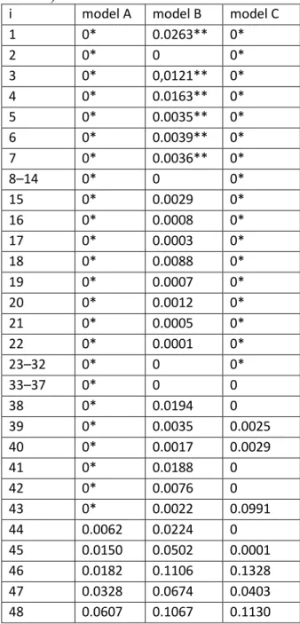
2.1.5. Observed latency of Lyme infection 160
To build a lag model used further in our research (please refer to Model II. A) we 161
determined the lags between tick bites and the first manifestations sampled from the 162
serological registration forms of the Hungarian National Reference Laboratory of 163
Bacterial Zoonoses from the period of March 2012–August 2012. Less than the 10% of 164
the serological registration forms contained both the data of the time of tick bites and 165
the appearance of the EM symptoms (n=26). Since most of the cases appeared 2-3 166
weeks after the tick bite it is plausible that these symptoms belonged to the early 167
manifestation forms (e.g. EM, neuroborreliosis). A lag model, forming a lognormal-like 168
shape, was built by approximating the observed lags between tick bites and onsets of the 169
early manifestation form (Fig 1.). Model values were found to be negligible after the 170
ninth week, therefore we used the first nine weeks later on.
171
2.2. Modeling method 172
2.2.1. Model overview 173
A two-phase model was built to estimate relative Lyme borreliosis incidence (LB) as an 174
output from two input parameters that are week number (n) (started from January) and 175
weekly average of the daily mean temperatures (T). All the other (hidden) parameters, 176
such as holiday multiplier (HM), tick activity (A), and biting activity (BA), are 177
calculated by the model from these two inputs. The reason of building a two-phase 178
model instead of a one-phase one was our aim to improve model reliability by a two- 179
phase calibration. The structure of the model and the sources of calibration are shown in 180
Fig 2. All the parameters of the model have weekly temporal resolution. For using the 181
model for real-time prediction one has to have the input T parameter for all the 52 182
6 weeks before the studied week.
183
Script (function) of the model that can be run in R statistical software (R Core 184
Team 2017) is provided (Github 2019). Although among the input T values all the 185
internal parameters and weights can be passed to the function, calibrated values are 186
automatically used if they are not specified.
187
The first phase of the model (hereinafter Model I) is able to estimate tick activity 188
and therefore the result of Model I may have relevance without the second phase 189
(hereinafter Model II), i.e. for estimating tick density, tick-borne encephalitis incidence 190
or the incidence of other tick-borne diseases. Model I is a composite of two models: the 191
first one (hereinafter season 1) is responsible for the tick activity in the first half of the 192
year, the second one (hereinafter season 2) is responsible for that of the second half of 193
the year. The division of the year is not strict and is done automatically by the model 194
based on n and T values. The calculation of season 1 is more complex than that of 195
season 2, since season 1 takes the size of the active population – those ticks that have 196
not yet bitten – into consideration. Tick activity is calculated by summarizing season 1 197
and season 2, since they may overlap each other (Eq. 1).
198
𝐴𝑛 = 𝐴𝑛𝑠𝑒𝑎𝑠𝑜𝑛 1+ 𝐴𝑛𝑠𝑒𝑎𝑠𝑜𝑛 2 (Eq. 1) 199
Since I. ricinus uses ambush strategy for host finding (Sonenshine 1991), the 200
probability of the encounter and therefore that of the disease transmission, depends not 201
only on tick activity but on human activity as well. Hence, infection is not directly 202
linked to tick activity but to the human-tick interaction. Biting activity is calculated 203
from tick activity and holiday multiplier (Eq. 2).
204
𝐵𝐴𝑛 = 𝐴𝑛 ∗ 𝐻𝑀𝑛 (Eq. 2)
205
Model II is able to estimate relative Lyme borreliosis incidence from biting activity. If 206
its input is available, Model II can be calibrated and used independently form Model I.
207
Model II has three alternative versions (model A, model B, and model C) that differ 208
from each other in terms of the calibration method. Model I and Model II is now going 209
to be explained in detail. After that model calibration will be discussed.
210
2.2.2. Model I, season 1 211
Season 1 in Model I inevitably contains the spring activity of adult ticks, but the nymph 212
activity seems to be dominant in causing Lyme infection from spring to late summer in 213
Hungary (Egyed et al. 2012). Tick activity in season 1 is estimated according to that 214
hard ticks take one blood meal per life stage (Randolph 2004) and therefore not all the 215
nymphs (and adults) are unfed in a certain week. Hence, the value of population entirety 216
(or active population, P) has to be taken into account and continuously diminished week 217
by week. P means the size of the active, unfed population (those ticks that ambush to 218
bite) between 0 and 1, where P of the first week of the year is 1 (Eq. 3).
219
𝑃 ∈ [0,1]; 𝑃1 = 1 (Eq. 3)
220
Tick activity is the function of the potential activity of the entire population 221
(temperature dependent activity, TDA) and the size of the actual unfed tick population.
222
The model calculates the active population of the current week iteratively from TDA 223
and the active population of the previous week. The subtrahend (S) is estimated from 224
7 the tick activity and a weight parameter (δ) (Eq. 4, Eq. 5).
225
𝑃𝑛 = { 0, 𝑖𝑓 𝑃𝑛−1− 𝑆𝑛−1 ≤ 0
𝑃𝑛−1− 𝑆𝑛−1, 𝑖𝑓 𝑃𝑛−1 − 𝑆𝑛−1 > 0 (Eq. 4) 226
𝑆𝑛 = 𝑇𝐷𝐴𝑛∗ 𝛿 (Eq. 5)
227
TDA means potential activity of the ticks that is dependent on temperature but 228
independent on the population size. Therefore, TDA means the tick activity that can be 229
measured if none of the specimens have been fed yet (if P=1). TDA is calculated from 230
the input temperature value and is based on a left-skewed lognormal distribution with 231
axis (α) that separates the lognormal distribution in the left side and the constant 0 232
function in the right side. The lognormal distribution has a mean (μ) and standard 233
deviation value (σ) and is multiplied with a factor (c) and then is increased with another 234
factor (d). The input of the lognormal distribution is the difference of T and α. TDA 235
starts to have a non-zero value when the temperature is above 5 °C in two consecutive 236
weeks (Eq. 6).
237
𝑇𝐷𝐴𝑛 = {
0, 𝑖𝑓 𝑇𝑛 ≥ 𝛼 ∨ 𝑇𝑛 ≤ 5 ∨ (𝑛 ≠ 1 ∧ 𝑇𝑛−1≤ 5)
𝑐 ∗ 1
(𝛼−𝑇𝑛)∗√2𝜋∗𝜎∗ 𝑒− (𝑙𝑛(𝛼−𝑇𝑛)−𝜇)2
2𝜎2 + 𝑑, 𝑒𝑙𝑠𝑒 (Eq. 6) 238
Tick activity (A) is calculated by the multiplication of TDA with the population entirety 239
(P) as shown in Eq. 7.
240
𝐴𝑛 = 𝑃𝑛∗ 𝑇𝐷𝐴𝑛 (Eq. 7)
241
Although TDA is usually a positive number (except in early spring and when the 242
temperature is greater than the axis), A is going to constantly be 0 after the week when 243
the P starts to be 0 (since all the specimens have been fed). Since the end of season 1 244
and the beginning of season 2 are not directly related to each other there may be a 245
period in summer when both of them or none of them have positive value.
246
2.2.3. Model I, season 2 247
The model of season 2 is simpler than that of season 1 since no population is taken into 248
account. It is thought that not the exhausted population but the cold temperature 249
together with the change of photoperiod has impact on the finishing of season 2, and 250
therefore there is no need to build a more complex model. Hence, TDA and A are 251
synonyms of each other in case of season 2 and P is set to be always 1. Tick activity is 252
calculated in a similar way to the equation shown in Eq. 6, except the conditions of the 253
two branches. In addition to that the temperature must be lower than the axis and greater 254
than 5 °C, A has a positive value from a certain week. This positive period begins when 255
the temperature drops below 20 °C (after the warmest week of the year and after the 28.
256
week) (Eq. 8). Since in case of real-time prediction the start of the period cannot be 257
calculated from the temperature values of the studied year, one can estimate maximum 258
temperature from the previous 52 weeks.
259
8 𝐴𝑛 =
260 {
0, 𝑖𝑓 𝑇𝑛 ≥ 𝛼 ∨ 𝑇𝑛 ≤ 5 ∨ max𝑖=1..52𝑇𝑖 ∉ ⋃𝑖=1..𝑛𝑇𝑖∨ n ≤ 28 ∨ ∀𝑖 ∈ [29, 𝑛]: 𝑇𝑖 ≥ 20
𝑐 ∗ 1
(𝛼−𝑇𝑛)∗√2𝜋∗𝜎∗ 𝑒− (ln(𝛼−𝑇𝑛)−𝜇)2
2𝜎2 + 𝑑, 𝑒𝑙𝑠𝑒 261
(Eq. 8) 262
2.2.4. Model II 263
Model II has the capability to estimate the LB based on the sum of the product of BA 264
and the weight factor (ω) of some of the previous weeks. The three versions of Model II 265
use different number of weeks. While model A uses exactly 9 weeks, model B and C 266
are able to use much more data and the exact number of the important weeks is gained 267
during the model calibration. The difference is detailed in the next chapter. To be 268
consistent in mathematical terms ω=0 weights are used when a model cannot calculate 269
with that certain week. Hence, all the three models have the similar equation (Eq. 9).
270
𝐿𝐵𝑛 = ∑𝑖=1..52(𝐵𝐴𝑛−53+𝑖∗ 𝜔𝑖) (Eq. 9) 271
2.3. Model calibration 272
The model was calibrated with input data averaged in the 11 years long period of 1998–
273
2008. Therefore, future prediction needs input data from a similarly long period. In case 274
of prediction with input data available from a shorter period (especially in case of real- 275
time prediction) the model has to be recalibrated.
276
The advantage of the two-phase model is that it has the possibility to calibrate 277
the model in two independent phases. In addition to the model inputs and the expected 278
output, we estimated BA that is a hidden parameter of the model. BA was approximated 279
by TBE data as proxy using a one-week shift (Eq. 10), since, in contrast to TBE, the 280
distribution of I. ricinus biting activity in weekly resolution is not known. Prodromal 281
symptoms of TBE appears about one week after tick bite and in general persist to the 282
second week before the neurological symptoms appear in the third week. Thus, shifting 283
TBE by one week may provide a well-established estimation of BA. In contrast to TBE, 284
using LB for calibration of BA would be less straightforward due to the complex and 285
multiphase nature of the manifestations of Lyme borreliosis infection.
286
𝐵𝐴𝑛 = 𝑇𝐵𝐸𝑛+1 (Eq. 10)
287
In case of Model II the so called model A was calibrated by using the observed latency 288
according to the serological application forms (in detail see Chapter 2.1.5). For 289
calibrating Model I, and Model II versions called B and C Solver add-in of Microsoft 290
Excel 2010 was used. Solver can find optimal solution (reduce the error of the model) 291
by adjusting parameters, subject to constraints. We used Generalized Reduced Gradient 292
nonlinear optimization from the several alternative optimization methods that Solver 293
provides. In case of Model I Solver calibrated 11 parameters simultaneously that are the 294
weight parameter (δ), and axis (α), mean (μ), standard deviation (σ), multiplier (c) and 295
difference (d) in case of season 1 and season 2. The set objective of the calibration was 296
to reduce the sum of squared errors of prediction (SSE) of tick activity (A). It should be 297
noted that calibration with such a high number of parameters has difficulties in case of 298
any automatic calibration processes. Therefore, iteratively more and more parameters 299
had been included in the calibration before the final calibration was done to ensure that 300
9 Solver finds the best solution not a local extreme value of SSE.
301
In case of Model II the set objective was to reduce the sum of squared errors of 302
prediction (SSE) of LB while changing the values of the weight factors (ω). In case of 303
model B all the 52 ω values were adjusted and in case of model C only 20 values were 304
adjusted (ω33 .. ω52). Both of the models were calibrated from the start stage that was 305
similar to model A. Thus, Solver could find optimal solution in spite of the fact that 306
52/20 parameters are not few to work with simultaneously. Model B is logically 307
incorrect since it is able to give non-zero values to ωi, where i is near to zero. This 308
means that the model uses the BA data from almost a year before the studied week 309
which is done because those data from the far past are statistically correlated to the data 310
of the near future (the next weeks) in all likelihood. Hence we suggest preferring model 311
C to model B since the former one uses only the real past for estimating LB.
312
3.RESULTS
313
3.1. Model calibration results 314
Weight parameter (δ) of Model I was calibrated to be 0.0078, while the other calibrated 315
parameters can be found in Table 2. Equations of the lognormal distribution of season 1 316
and season 2 (Eq. 6, Eq. 8) are now updated with the calibrated parameters (Eq. 11, Eq.
317
12).
318
𝑇𝐷𝐴𝑛 = {
0, 𝑖𝑓 𝑇𝑛 ≥ 26.3302 ∨ 𝑇𝑛 ≤ 5 ∨ (𝑛 ≠ 1 ∧ 𝑇𝑛−1 ≤ 5) 82.7165 ∗(26.3302−𝑇 1
𝑛)∗√2𝜋∗0.4804∗ 𝑒− (ln(26.3302−𝑇𝑛)−2.0337)2
2∗0.48042 , 𝑒𝑙𝑠𝑒 (Eq.
319
11) 320
𝐴𝑛 = 321
{
0, 𝑖𝑓 𝑇𝑛 ≥ 123.8382 ∨ 𝑇𝑛 ≤ 5 ∨ max𝑖=1..52𝑇𝑖 ∉ ⋃𝑖=1..𝑛𝑇𝑖∨ n ≤ 28 ∨ ∀𝑖 ∈ [29, 𝑛]: 𝑇𝑖 ≥ 20 6.8409 ∗(123.8382−𝑇𝑛1)∗√2𝜋∗0.0145∗ 𝑒− (ln(123.8382−𝑇𝑛)−4.7124)2
2∗0.01452 + 0.4931, 𝑒𝑙𝑠𝑒 322
(Eq. 12) 323
Calibration results of Model II can be seen in Table 3. The zero values that were not 324
calibrated but fixed are marked. Sums of the weights should be near 1. Sums of squared 325
errors of prediction (SSE) of relative Lyme borreliosis incidence can be found in Table 326
3 for making a comparison between the three models. Note that the set objective of 327
Solver was to minimize SSE in case of model B and model C. Model A seems to be 328
worse than model B and C in one order of magnitude. Model C is found to be the best 329
of the three model version, although model B (with 52 adjustable parameters instead of 330
20) had the ability to take precedence over model C. This result shows that Solver found 331
local extreme during calibration of model B. The authors suggest using model C instead 332
of the other ones. The provided R function (Github 2019) uses automatically model C 333
and the calibrated parameters and weights if they are not passed to the function.
334
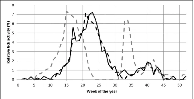
3.2. Prediction of relative biting activity 335
The modeled distribution of relative tick biting activity (BA; Fig 3) in the reference 336
period is bimodal with a major peak in the second part of May and a clear but minor 337
10 peak in late September. According to the similar run of the tick activity curves of the 338
model and the calibration data, the model was calibrated well. The prediction to the 339
period of 2081–2100 shows that the two parts of the biting activity curve will be 340
separated more markedly. This finding is consistent with the expectations. Maximum of 341
the activity is predicted to be shifted 8 weeks earlier, while the tick season may start 6-7 342
weeks earlier than in the reference period. Significant prolongation of the fall season is 343
not predicted, therefore the whole tick season seems to become 6-7 weeks longer in the 344
future. However, if summer diapause is taken into account, the length of the period 345
when ticks are effectively active will not be changed. The fall local maximum may shift 346
from the 40th to the 33rd–34th weeks and become more pronounced according to the 347
prediction. In terms of its scale, the fall maximum may almost reach the spring one 348
causing bimodality of relative tick activity become more explicit.
349
3.3. Prediction of relative lyme borreliosis incidence 350
The three predictions to the reference period (Fig 4, black lines) prove the findings of 351
the calibration about model errors. Model B and model C, those that were trained 352
algorithmically, fit better to the observed Lyme borreliosis curve than model A does.
353
While prediction of model B and that of model C are largely similar to each other, 354
advantage of model C over the other one can be seen in the weeks 24–29. Unimodal 355
annual distribution of the Lyme borreliosis incidences are obviously shown by all the 356
three predictions.
357
Future predictions (Fig 4, gray lines) demonstrate the bimodalization of the 358
annual incidence distribution by the end of the 21st century. The bimodal distribution 359
shows similar characteristics to that of the predicted future relative tick biting activity, 360
especially in case of model A. All the three models predict the elongation of the total 361
Lyme borreliosis season by about 8 weeks. However, the effective length of the season 362
seems to be shortened in the future by some weeks, due to the narrowing of the main 363
curve. Although predictions to the future and the reference period are somewhat similar 364
to each other after the 38th week, they are largely different before. From 26th to 34th 365
weeks LBs are close to zero, while the period of the weeks no. 13–24 may be highly 366
endangered by Lyme borreliosis. The maximum relative incidence will shift from the 367
currently observed 27th week to the 18th–19th weeks, according to the predictions. The 368
three models agree that fall local maximum will occur in the 36th week but the LB is 369
predicted to be one and a half time higher by model A than by model B and C. With 370
reference to the previously written calibration results, we may conclude that model A is 371
performing poorly for the future period too and overestimates maxima of LB.
372
4.DISCUSSION
373
4.1. Model advantages and improvements 374
Although a lot of model parameters had been calibrated by Solver simultaneously in 375
case of Model I. and Model II., calibration found optimal solution in both cases and the 376
calibrated model predicted the annual distribution of Lyme borreliosis incidences with 377
low error values. Hence, the complexity of the model is thought to be not too high but 378
not too low either, since the model can estimate the expected output parameter (i.e. the 379
relative Lyme borreliosis incidence of a certain week) well. An important advantage of 380
our model is that it needs temperature data only as input parameter in addition to the 381
11 week numbers (c.f. Wu et al.'s (2010) model on I. scapularis population). Observed or 382
predicted daily/weekly temperatures are easily available data with high horizontal and 383
temporal resolution for a great part of the world and for a wide range of past and future 384
time periods. Therefore, our modeling framework is thought to be a not input-intensive, 385
easy-to-use estimator of Lyme borreliosis infection.
386
Our framework contains several innovations in modeling the annual distribution 387
of Lyme borreliosis incidence: (1) the model is calibrated in two phases, where the first 388
phase describes the biting activity of ticks; (2) human-tick interaction is taken into 389
account and estimated using camping guest night data (c.f. Šumilo et al. 2008; Pfäffle et 390
al. 2013); (3) the spring and fall seasons are modeled separately due to their different 391
activity patterns and their different dependence on climate; (4) a simple and 392
straightforward population dynamics module is implemented in Model I, season 1.
393
Although it is clear that activity patterns of the two modeled seasons differ from each 394
other in the region of our study, it is not yet known if they are related only with the 395
different seasonal activity of the nymph and adult ticks. Although findings of Hornok 396
and Farkas (2009) and Egyed et al. (2012) for Hungary, and also Randolph et al. (2002), 397
Takken et al. (2016) and Cayol et al. (2017) for other regions cannot strengthen our 398
supposition, there is evidence on the dominance of nymphs in spring and that of the 399
adults in fall (Trájer and Földvári unpublished data). Since adults are active in spring as 400
well (Randolph et al. 2002; Hornok and Farkas 2009; Egyed et al. 2012), Model I, 401
season 1 was built to deal with nymphs and adults jointly. However, the higher infection 402
rate of the nymphs (Olsén et al. 1995) and their more efficient Borrelia transmission 403
due to their less perceptibility support that the population dynamics module based on 404
the questing behavior of nymphs was implemented in Season 1. This module can 405
describe the abundance-meditated probability of questing, similarly to the model of 406
Dobson et al. (2011).
407
Even if Model I cannot substitute for tick flagging, the indirect biting activity 408
data derived from tick-borne encephalitis used in the our study may be more suitable for 409
analyzing temperature-related seasonal tick activity patterns than field surveys due to 410
their high temporal resolution, accessibility, and higher sample size. Although from an 411
unconventional aspect (i.e. backward conclusion from incidence data), our model 412
highlights the significance of the nosocomial surveillance systems. Determination of the 413
exact time of tick bite based on the notification system of Lyme infection is biased, 414
since (1) erythema migrans begins after a delay of 3 to 30 days after tick bite (in 415
average 2 weeks latency); (2) the time of the human-tick encounter that enable tick bite 416
is often not known exactly; (3) the reported Lyme borreliosis cases contain the mixture 417
of different stages that have different latencies; (4) the notification probability of the 418
different stages is different. Our modeling framework provides a simple workaround 419
that eliminates these uncertainties. Biting activity is calculated from temperature, week 420
number and the probability of human-tick interaction (i.e. holiday multiplier), and is 421
calibrated by the much more consistent, reliable and predictable tick-borne encephalitis 422
(Gray et al. 2009) instead of Lyme borreliosis data (c.f. the suggestion of Bózsik (2004) 423
on the use of tick-borne encephalitis series to predict Lyme borreliosis series). The 424
modeling framework needs another calibration method in countries without tick-borne 425
encephalitis incidence. Three different latency models are then used to convert biting 426
activity series to LB series, among them two models are calibrated automatically. These 427
enhancements ensure that biting activity is highly independent from Lyme borreliosis 428
incidences and is calibrated with low uncertainty. The predicted annual distribution of 429
biting activity in the reference period is highly similar to the results of field studies 430
(Széll et al. 2006; Egyed et al. 2012; Trájer and Földvári unpublished data).
431
12 4.2. Interpretation of predictions
432
According to our results, start of the tick biting activity and Lyme borreliosis season, 433
length of the season, and other seasonal characteristics of the annual distribution are 434
highly sensitive to temperature, and hence, to climate change. Our findings underpin 435
those of previous researches on the impact of climate on the vector (e.g. Lindgren et al.
436
2000; Gray et al. 2009; Jaenson and Lindgren 2011; Trájer et al. 2013a; Li et al. 2016), 437
the disease (Jaenson and Lindgren 2011; Li et al. 2016), and the bacteria Borrelia 438
burgdorferi (Estrada-Peña et al. 2011). Hornok and Farkas (2009) found, however, that 439
the spring timing of the peak activity of I. ricinus was unaffected by the warm weather 440
of 2007 in the Hungary. It has been observed that the increasing length of the vegetation 441
period elongated the Lyme borreliosis season in the 2000's in Hungary (Trájer et al.
442
2013b), which trend is predicted by our model to continue in the future.
443
Although our model might be biased and its future prediction might be 444
inaccurate, the significant change of the annual distribution is clear and inevitable. Such 445
change of the climatic patterns may also cause future shift in the geographical 446
distribution of I. ricinus (Lindgren et al. 2000; Jore et al. 2014; Sormunen et al. 2016; Li 447
et al. 2016) and its close relative, the blacklegged tick, Ixodes scapularis (Estrada-Peña 448
2002; Brownstein et al. 2003; Ogden et al. 2008), which has already been observed in 449
the last decades (Daniel 1993; Daniel and Dusbabek 1994; Lindgren et al. 2000). Please 450
refer to Estrada-Peña (2008) for a critical review of these findings. It is an open 451
question how climate change will trigger the northward move of Mediterranean tick 452
species, however, the European range and distribution of the population of such 453
Mediterranean tick species like of Dermacentor reticulatus shows a stable increasing 454
trend in Europe and the Carpathian Basin (Földvári et al. 2016).
455
Since spring is predicted to be warmer, and the summer will be drier and hotter 456
in Hungary according to the climate models (Pieczka et al. 2018), the forecasted 457
bimodal distribution of tick biting activity and Lyme borreliosis incidence is consistent 458
with our expectations. Our findings underpinned that the apparent contradiction 459
between the unimodal distribution of Lyme borreliosis and bimodal distribution of tick- 460
borne encephalitis might be the result of the different incubation periods of the organic 461
manifestations rather than the consequence of the different seasonal infection rate or the 462
difference of the vector species.
463
Extreme events (e.g. heat) might become more intensive and frequent in the 464
future (Bai et al. 2016), which trend is attributed to global climate change by 465
researchers (Göndöcs et al. 2018) and stakeholders (Malatinszky et al. 2013) as well.
466
Their increasing frequency creates an uncertain basis for environmental predictions 467
(Şen 2018). Therefore, understanding and, if necessary, reducing their impact is an 468
important topic of climate change studies (Birkmann and Welle 2015). Our framework 469
can predict the tick biting activity in the periods of extreme heat more reliably than the 470
models that are prone to overestimate it (e.g. Cat et al. 2017). Previous findings on the 471
accelerated phenology of ticks in the warming future climate (Süss et al. 2008; Levi et 472
al. 2015; Li et al. 2016) is strengthen by our results.
473
4.3. Usability of the model and limitations of the result interpretation 474
Model I is suggested to be used to calculate tick biting activity (and indirectly tick 475
activity, tick density, and more indirectly relative incidence of tick-borne encephalitis), 476
while the authors recommend using Model II to estimate relative Lyme borreliosis 477
incidence (and indirectly absolute Lyme borreliosis incidence). The provided R script 478
13 (Github 2019) is thought to enhance the usability of our model since it need only 479
weekly temperature series and returns the result of both modeling phases (relative biting 480
activity, relative Lyme borreliosis incidence). It provides an effective tool for those who 481
need quick prediction (by using default, calibrated parameters) and for those, as well, 482
who have recalibrated the model and could pass the recalculated parameters to the 483
function.
484
Despite that some other environmental factors (e.g. precipitation, humidity) 485
might have role on determining the distribution of Lyme borreliosis incidence 486
(Randolph 2009; Jore et al. 2014; Cat et al. 2017), we presented a highly input- 487
extensive, simple modeling framework that uses, among the calibration data, only 488
temperature and week number as input parameters. Since humidity is highly affected by 489
vegetation, nearness of water bodies, and urbanization level, fine resolution humidity 490
data that are free from these biases is hardly accessible. Since both the present (i.e.
491
reference period) and future predictions of our model meet our previous expectations, 492
we conclude that the observed summer decrease of the Lyme borreliosis incidence is not 493
necessarily or solely the consequence of the low summer precipitation or reduced 494
humidity as many author claimed (e.g. Schauber et al. 2005; Ostfeld et al. 2006). Tick 495
population dynamics, which was applied in Model I, season 1, can be an alternative 496
explanation of the observed patterns of the summer distribution, at least in Hungary.
497
Although the decreasing numbers of questing ticks might be the consequence of several 498
factors, such as increased mortality due to changing meteorological conditions, our 499
model confirmed that one and major determinant of the decrease is the loss of hungry 500
tick population due to their previous bite.
501
Climate is not the only one important environmental factor which can have 502
impact on tick-borne diseases in Hungary. It was also found that inexperienced farmers 503
who have a lower rate of preventive actions are likely to experience greater exposure to 504
tick bites in Hungary (Li et al. 2018). It cannot be excluded that the reduced use of 505
pesticides in tick control in the urban environment also influenced the abundance of the 506
urban tick populations in the last decades in Hungary.
507
Since the main objectives of model building includes simplification of reality by 508
making assumptions and generalizations, its tradeoffs are amplified when reduction of 509
model complexity and the number of input parameters is aimed. Therefore, we should 510
list the weaknesses and limitations of the model:
511
1) camping guest night data can serve only as a proxy of human outdoor 512
activities: its annual distribution may differ from that of all the outdoor activities and 513
cannot cover people of occupational risk groups, e.g. foresters;
514
2) complex ecology of I. ricinus can approximated but not fully described if no 515
other environmental factors than temperature are considered. Although temperature is 516
correlated to photoperiodicity, relative humidity and saturation deficit, it cannot replace 517
the other abiotic factors. For simplicity, we must accept the improper assumption that 518
temperature can describe the tick's annual distribution;
519
3) the tick-borne encephalitis data used for calibration is limited to part of the 520
geographic range of I. ricinus. Hence, other data source is required for calibration in 521
such territories. Surveillance data is prone to several type of biases, including 522
geographical bias, reporting bias and inaccurate diagnosis etc.;
523
4) both Lyme borreliosis and tick-borne encephalitis data may suffer from the 524
difficulties in case definition criteria, latency of infection, great variability of human 525
response and that of the pathogenicity of the agents;
526
14 5) instead of a reasonable but more complex birth-rate distribution, all 527
individuals enter the population at the beginning of the year in our model, which cannot 528
describe the real nature of population dynamics of the species;
529
6) the used population dynamics approach (Model I, season 1) can only partly 530
explain the observed abundance changes, since, beyond the disappearing of active 531
individuals due to successful feeding, natural mortality and diapause are not taken into 532
account.
533
Predicted annual distributions of both tick biting activity and relative Lyme 534
borreliosis incidence to the reference and future periods are in agreement with literature 535
(e.g. Gray 2008; Gray et al. 2009; Jaenson and Lindgren 2011; Zöldi et al. 2013; Li et 536
al. 2016). The forecasted remarkable summer decrease of tick biting activity and Lyme 537
incidence in the future underpins the findings of Burtis et al. (2016) on I. scapularis 538
activity. From the predicted changes in the annual distribution of relative Lyme 539
incidence the absolute annual incidence cannot be estimated directly. Note that 540
according to some researchers (e.g. Shope 1991) absolute number of incidences might 541
decrease in the future. Our framework, similarly to other climate-based modeling 542
approaches, is sensitive to the selection of the emission scenario and regional climate 543
model (c.f. Cat et al. 2017). However, compared with the less complex models that are 544
based on additive warming terms, there is a need for such regional climate model driven 545
approaches to better understand the future of the disease (Li et al. 2016).
546
Our predictions are extrapolations in terms of the climatic space. Since tick 547
biting activity in such climatic conditions that are predicted to occur in Hungary in 548
2081–2100 is not well studied yet, our future predictions should be interpreted with 549
caution and need further evaluation. More research on the future seasonality of Lyme 550
incidence and I. ricinus activity is needed for the regions where hot summers may limit 551
tick abundance and activity (i.e. Southern Europe).
552
5.CONCLUSION
553
The presented framework with low number of inputs on modeling the seasonality of 554
Lyme borreliosis incidences enables predicting the annual distribution of Ixodes ricinus 555
tick's biting activity and Lyme borreliosis in two cascading phases, using only the easily 556
accessible weekly temperature data and week numbers as input parameters. Based on 557
the implemented innovations incorporated in our model (i.e. two phases; population 558
dynamics model of the spring season; tick-borne encephalitis series as a proxy for tick 559
biting activity during the calibration; human-tick interaction approximated by camping 560
data), it provides a simple workaround for several known issues of modeling Lyme 561
seasonality, including the hardly available data on tick activity. According to the 562
prediction to the future period of 2081–2100 based on MRI CGCM regional climate 563
model and A1B emission scenario, climate change may significantly alter both the 564
annual distribution of I. ricinus activity and that of the Lyme borreliosis incidences.
565
While the currently unimodal annual distribution of Lyme borreliosis is predicted to 566
become bimodal with a long summer pause and a spring maximum shifted 8 weeks 567
earlier, the bimodality of I. ricinus activity may also become more expressed.
568
ACKNOWLEDGEMENTS
569
The authors would like to express their gratitude to Gábor Földvári (Department of Parasitology 570
and Zoology, University of Veterinary Medicine Budapest, Hungary) for his comments on an 571
15 early version of this paper. The project was supported by the GINOP-2.3.2-15-2016-00019 572
grant.
573
REFERENCES
574
Akhtar MK, Simonovic SP, Wibe J, MacGee J (2019): Future realities of climate 575
change impacts: an integrated assessment study of Canada. Int J Global Warm 576
17(1): 59–88. http://dx.doi.org/10.1504/IJGW.2019.096761 577
Aleixandre-Tudó JL, Bolaños-Pizarro M, Aleixandre JL, Aleixandre-Benavent R 578
(2019): Current trends in scientific research on global warming: a bibliometric 579
analysis. Int J Global Warm 17(2): 142–169.
580
http://dx.doi.org/10.1504/IJGW.2019.097858 581
Bai H, Dong X, Zeng S, Chen J (2016): Assessing the potential impact of future 582
precipitation trends on urban drainage systems under multiple climate change 583
scenarios. Int J Global Warm 10(4): 437–453.
584
http://dx.doi.org/10.1504/IJGW.2016.079776 585
Birkmann J, Welle T (2015): Assessing the risk of loss and damage: exposure, 586
vulnerability and risk to climate-related hazards for different country 587
classifications. Int J Global Warm 8(2): 191–212.
588
http://dx.doi.org/10.1504/IJGW.2015.071963 589
Bózsik BP (2004): Prevalence of Lyme borreliosis. Lancet 363: 901.
590
http://dx.doi.org/10.1016/S0140-6736(04)15756-5 591
Brownstein JS, Holford TR, Fish D (2003): A Climate-Based Model Predicts the Spatial 592
Distribution of the Lyme Disease Vector Ixodes scapularis in the United States.
593
Environ Health Perspect 111(9): 1152–1157. http://dx.doi.org/10.1289/ehp.6052 594
Burtis JC, Sullivan P, Levi T, Oggenfuss K, Fahey TJ, Ostfeld RS (2016): The impact 595
of temperature and precipitation on blacklegged tick activity and Lyme disease 596
incidence in endemic and emerging regions. Parasit Vectors 9(1): 606.
597
http://dx.doi.org/10.1186/s13071-016-1894-6 598
Cat J, Beugnet F, Hoch T, Jongejan F, Prangé A, Chalvet-Monfray K (2017): Influence 599
of the spatial heterogeneity in tick abundance in the modeling of the seasonal 600
activity of Ixodes ricinus nymphs in Western Europe. Exp Appl Acarol 71(2):
601
115–130. http://dx.doi.org/10.1007/s10493-016-0099-1 602
Cayol C, Koskela E, Mappes T, Siukkola A, Kallio ER (2017): Temporal dynamics of 603
the tick Ixodes ricinus in northern Europe: epidemiological implications. Parasit 604
Vectors 10(1): 166. http://dx.doi.org/10.1186/s13071-017-2112-x 605
Daniel M, Dusbabek F (1994): Micrometeorological and microhabitat factors affecting 606
maintenance and dissemination of tick-borne diseases in the environment. In:
607
Sonenshine DE, Mather TN (eds.): Ecological dynamics of tick-borne zoonoses.
608
New York, NY, USA: Oxford University Press.
609
Daniel, M. (1993). Influence of the microclimate on the vertical distribution of the tick 610
Ixodes ricinus (L.) in central Europe. Acarologia 34(2): 105–113.
611
Dobson ADM, Finnie TJR, Randolph SE (2011): A modified matrix model to describe 612
the seasonal population ecology of the European tick Ixodes ricinus. J Appl Ecol 613
48(4): 1017–1028. http://dx.doi.org/10.1111/j.1365-2664.2011.02003.x 614
Egyed L, Élő P, Sréter-Lancz Z, Széll Z, Balogh Z, Sréter T (2012): Seasonal activity 615
and tick-borne pathogen infection rates of Ixodes ricinus ticks in Hungary. Ticks 616
Tick Borne Dis 3: 90–94. http://dx.doi.org/10.1016/j.ttbdis.2012.01.002 617
Epstein PR (1999): Climate and health. Science 285(5426): 347–348.
618
http://dx.doi.org/10.1126/science.285.5426.347 619
16 Estrada-Peña A (2002): Increasing habitat suitability in the United States for the tick 620
that transmits Lyme disease: a remote sensing approach. Environ Health 621
Perspect 110: 635–640. http://dx.doi.org/10.1289/ehp.02110635 622
Estrada-Peña A (2008): Climate, niche, ticks, and models: what they are and how we 623
should interpret them. Parasitol Res 103(Suppl 1): 87–95.
624
http://dx.doi.org/10.1007/s00436-008-1056-7 625
Estrada-Peña A, Ortega C, Sánchez N, DeSimone L, Sudre B, Suk JE, Semenza JC 626
(2011): Correlation of Borrelia burgdorferi Sensu Lato Prevalence in Questing 627
Ixodes ricinus Ticks with Specific Abiotic Traits in the Western Palearctic. Appl 628
Environ Microb 77(11): 3838–3845. http://dx.doi.org/10.1128/AEM.00067-11 629
Földvári G, Farkas R (2005): Ixodid tick species attaching to dogs in Hungary. Vet 630
Parasitol 129: 125–131.
631
Földvári G, Siroky P, Majoros G, Szekeres S, Sprong H (2016): Dermacentor 632
reticulatus: a vector on the rise. Parasite Vector 9: 314.
633
https://doi.org/10.1186/s13071-016-1599-x 634
Github (2019): R script of the model. URL:
635
github.com/bfakos/lyme_model/blob/master/Supplementary_material_S1.r 636
Göndöcs J, Breuer H, Pongrácz R, Bartholy J (2018): Projected changes in heat wave 637
characteristics in the Carpathian Basin comparing different definitions. Int J 638
Global Warm 16(2): 119–135. http://dx.doi.org/10.1504/IJGW.2018.094552 639
Gray JS (2008): Ixodes ricinus seasonal activity: Implications of global warming 640
indicated by revisiting tick and weather data. Int J Med Microbiol 298(S1): 19–
641
24. http://dx.doi.org/10.1016/j.ijmm.2007.09.005 642
Haylock MR, Hofstra N, Klein Tank AMG, Klok EJ, Jones PD, New M (2008): A 643
European daily high resolution gridded data set of surface temperature and 644
precipitation for 1950–2006. J Geophys Res–Atmos 113(D20).
645
http://dx.doi.org/10.1029/2008JD010201 646
Hornok S, Farkas R (2009): Influence of biotope on the distribution and peak activity of 647
questing ixodid ticks in Hungary. Med Vet Entomol 23: 41–46.
648
http://dx.doi.org/10.1111/j.1365-2915.2008.00768.x 649
Hunter PR (2003): Climate change and waterborne and vector borne disease. J Appl 650
Microbiol 94(S1): 37–46. http://dx.doi.org/10.1046/j.1365-2672.94.s1.5.x 651
Jaenson TGT, Lindgren E (2011): The range of Ixodes ricinus and the risk of 652
contracting Lyme borreliosis will increase northwards when the vegetation 653
period becomes longer. Ticks Tick-borne Dis 2(1): 44–49.
654
http://dx.doi.org/10.1016/j.ttbdis.2010.10.006 655
Jaha IR, Ekumah EK (2015): Climate change, fish catch and premix fuel supply to 656
fishermen for sustainable livelihoods of coastal people in the central region of 657
Ghana. Int J Global Warm 8(4): 453–462.
658
http://dx.doi.org/10.1504/IJGW.2015.073050 659
Jore S, Vanwambeke SO, Viljugrein H, Isaksen K, Kristoffersen AB, Woldehiwet Z, 660
Johansen B, Brun E, Brun-Hansen H, Westermann S, Larsen IL, Ytrehus B, 661
Hofshagen M (2014): Climate and environmental change drives Ixodes ricinus 662
geographical expansion at the northern range margin. Parasit Vectors 7(1): 11.
663
http://dx.doi.org/10.1186/1756-3305-7-11 664
Levi T, Keesing F, Oggenfuss K, Ostfeld RS (2015): Accelerated phenology of 665
blacklegged ticks under climate warming. Phil Trans R Soc B 370(1665):
666
20130556. http://dx.doi.org/10.1098/rstb.2013.0556 667
Li S, Gilbert L, Harrison PA, Rounsevell MDA (2016): Modelling the seasonality of 668
Lyme disease risk and the potential impacts of a warming climate within the 669
17 heterogeneous landscapes of Scotland. J R Soc Interface 13(116): 20160140.
670
http://dx.doi.org/10.1098/rsif.2016.0140 671
Li S, Juhász‐Horváth L, Trájer A, Pintér L, Rounsevell MDA, Harrison PA (2018):
672
Lifestyle, habitat and farmers' risk of exposure to tick bites in an endemic area 673
of tick‐borne diseases in Hungary. Zoonoses Public Health 65(1): e248–e253.
674
http://dx.doi.org/10.1111/zph.12413 675
Lindgren E (1998): Climate change, tick-borne encephalitis and vaccination needs in 676
Sweden – a prediction model. Ecol Model 110(1): 55–63.
677
Lindgren E, Talleklint L, Polfeldt T (2000): Impact of climatic change on the northern 678
latitude limit and population density of the disease-transmitting European tick 679
Ixodes ricinus. Environ Health Perspect 108: 119–123.
680
http://dx.doi.org/10.1289/ehp.00108119 681
Lindgren E, Jaenson TG (2006): Lyme borreliosis in Europe: influences of climate and 682
climate change. epidemiology, ecology and adaptation measures. Copenhagen, 683
Denmark: World Health Organization.
684
Lindsay LR, Barker IK, Surgeoner GA, McEwen SA, Gillespie TJ, Robinson JT (1995):
685
Survival and development of Ixodes scapularis (Acari: Ixodidae) under various 686
climatic conditions in Ontario, Canada. J Med Entomol 32: 143–152.
687
http://dx.doi.org/10.1093/jmedent/32.2.143 688
Malatinszky Á, Ádám Sz, Saláta-Falusi S, Saláta D, Penksza K (2013): Planning 689
management adapted to climate change effects in terrestrial wetlands and 690
grasslands. Int J Global Warm 5(3): 311–325.
691
http://dx.doi.org/10.1504/IJGW.2013.055365 692
OEK (2013): Országos Epidemiológiai Központ. [National Center for Epidemiology].
693
URL: www.oek.hu [Last accessed: 03/01/2013].
694
Ofulla AVO, Gichere SK, Olado GO, Abuom PO, Anyona DN, Othero DM, Matano A- 695
S, Gelder FB, Dida GO, Ouma C, Owuor PO, Amayi JB, Kanangire CK (2016):
696
Effects of regional climate variability on the prevalence of diseases and their 697
economic impacts on households in the Lake Victoria basin of Western Kenya.
698
Int J Global Warm 10(1–3): 332–353.
699
http://dx.doi.org/10.1504/IJGW.2016.077899 700
Ogden NH, Bigras-Poulin M, O’Callaghan CJ, Barker IK, Lindsay LR, Maarouf A, 701
Smoyer- Tomic KE, Waltner-Toews D, Charron D (2005): A dynamic 702
population model to investigate effects of climate on geographic range and 703
seasonality of the tick Ixodes scapularis. Int J Parasitol 35: 375–389.
704
http://dx.doi.org/10.1016/j.ijpara.2004.12.013 705
Ogden NH, St-Onge L, Barker IK, Brazeau S, Bigras-Poulin M, Charron DF, Francis 706
CM, Heagy A, Lindsay LR, Maarouf A, Michel P, Milord F, O'Callaghan CJ, 707
Trudel L, Thompson RA (2008): Risk maps for range expansion of the Lyme 708
disease vector, Ixodes scapularis, in Canada now and with climate change. Int J 709
Health Geogr 7: 24. http://dx.doi.org/10.1186/1476-072X-7-24 710
Olsén B, Jaenson TG, Bergström S (1995): Prevalence of Borrelia burgdorferi sensu 711
lato-infected ticks on migrating birds. Appl Environ Microbiol 61(8): 3082–
712
3087.
713
Ostfeld RS, Canham CD, Oggenfuss K, Winchcombe RJ, Keesing F (2006): Climate, 714
deer, rodents, and acorns as determinants of variation in Lyme-disease risk.
715
PLoS Biol 4(6): e145. http://dx.doi.org/10.1371/journal.pbio.0040145 716
Ostfeld RS, Schauber EM, Canham CD, Keesing F, Jones CG, Wolff JO (2001): Effects 717
of acorn production and mouse abundance on abundance and Borrelia 718
18 burgdorferi infection prevalence of nymphal Ixodes scapularis ticks. Vector 719
Borne Zoonotic Dis 1: 55–63.
720
Pfäffle M, Littwin N, Muders SV, Petney TN (2013): The ecology of tick-borne 721
diseases. Int J Parasitol 43(12-13): 1059–1077.
722
Pieczka I, Pongrácz R, Bartholy J, Szabóné André K (2018): Future temperature 723
projections for Hungary based on RegCM4.3 simulations using new 724
Representative Concentration Pathways scenarios. Int J Global Warm 15(3):
725
277–292. http://dx.doi.org/10.1504/IJGW.2018.093121 726
R Core Team (2017): R: A language and environment for statistical computing. R 727
Foundation for Statistical Computing, Vienna, Austria. URL: www.R- 728
project.org.
729
Randolph SE (2009): Epidemiological consequences of the ecological physiology of 730
ticks. Adv Insect Physiol 37: 297–339.
731
Randolph SE (2004): Tick ecology: processes and patterns behind the epidemiological 732
risk posed by ixodid ticks as vectors. Parasitology 129(Suppl): S37–S65.
733
http://dx.doi.org/10.1017/S0031182004004925 734
Randolph SE, Green RM, Hoodless AN, Peacey MF (2002): An empirical quantitative 735
framework for the seasonal population dynamics of the tick Ixodes ricinus. Int J 736
Parasitol 32: 979–989. http://dx.doi.org/10.1016/S0020-7519(02)00030-9 737
Rizzoli A, Silaghi C, Obiegala A, Rudolf I, Hubálek Z, Földvári G, Plantard O, 738
Vayssier-Taussat M, Bonnet S, Spitalska E, Kazimirová M (2014): Ixodes 739
ricinus and its transmitted pathogens in urban and peri-urban areas in Europe:
740
new hazards and relevance for public health. Front Public Heal 2: 251.
741
http://dx.doi.org/10.3389/fpubh.2014.00251 742
Rogers DJ, Randolph SE (2006): Climate change and vector-borne diseases. Adv 743
Parasitol 62: 345–381. http://dx.doi.org/10.1016/S0065-308X(05)62010-6 744
Schauber EM, Ostfeld RS, Evans AS Jr (2005): What is the best predictor of annual 745
Lyme disease incidence: weather, mice, or acorns? Ecol Appl 15(2): 575–586.
746
http://dx.doi.org/10.1890/03-5370 747
Şen Z (2018): Noah and Joseph effects: floods and droughts under global warming. Int J 748
Global Warm 16(3): 347–364. http://dx.doi.org/10.1504/IJGW.2018.095390 749
Shope R (1991): Global climate change and infectious diseases. Environ Health 750
Perspect 96: 171–174. http://dx.doi.org/10.1289/ehp.9196171 751
Sonenshine DE (1991): Biology of Ticks, vol. 1. New York, NY, USA: Oxford 752
University Press.
753
Sormunen JJ, Klemola T, Vesterinen EJ, Vuorinen I, Hytönen J, Hänninen J, 754
Ruohomäki K, Sääksjärvi IE, Tonteri E, Penttinen R (2016): Assessing the 755
abundance, seasonal questing activity, and Borrelia and tick-borne encephalitis 756
virus (TBEV) prevalence of Ixodes ricinus ticks in a Lyme borreliosis endemic 757
area in Southwest Finland. Ticks and Tick-borne Diseases 7(1): 208–215.
758
http://dx.doi.org/10.1016/j.ttbdis.2015.10.011 759
Széll Z, Sréter-Lancz Z, Márialigeti K, Sréter T (2006): Temporal distribution of Ixodes 760
ricinus, Dermacentor reticulatus and Haemaphysalis concinna in Hungary. Vet 761
Parasitol 141(3–4): 377–379. http://dx.doi.org/10.1016/j.vetpar.2006.06.008 762
Šumilo D, Bormane A, Asokliene L, Vasilenko V, Golovljova I, Avsic-Zupanc T, 763
Hubalek Z, Randolph SE (2008): Socio-economic factors in the differential 764
upsurge of tick-borne encephalitis in central and Eastern Europe. Rev Med Virol 765
18(2): 81–95.
766