Anti-cyclical versus Risk-sensitive Margin Strategies in Central
Clearing
by Edina Berlinger, Barbara Dömötör, Ferenc Illés
C O R VI N U S E C O N O M IC S W O R K IN G P A PE R S
http://unipub.lib.uni-corvinus.hu/2894
CEWP 3 /201 7
1
Anti-cyclical versus Risk-sensitive Margin Strategies in Central Clearing
Edina Berlinger1 Associate Professor
Department of Finance, Corvinus University of Budapest Barbara Dömötör2
Assistant Professor
Department of Finance, Corvinus University of Budapest Ferenc Illés3
PhD-student
Department of Finance, Corvinus University of Budapest 24.05.2017
Abstract
We analyzed the effects of different margin strategies on the loss distribution of a clearinghouse during different crises. First, we developed a general one-period analytical model and proved the existence of a unique optimal margin which is not necessarily risk-sensitive even in a weaker sense. Then, we simulated the operation of a hypothetical clearinghouse active on the US stock futures market in the period 2008-2015. We found that anti-cyclical margin strategies might be optimal also for clearinghouses focusing on their micro-level financial stability, not only for regulators aiming to reduce systemic risk. Anti-cyclical margin strategies performed especially well in minor crises like Flash Crash.
JEL-codes G20, G28 Keywords
financial stability, clearinghouse, central counterparty, EMIR, agent-based simulation, stochastic dominance
1 edina.berlinger@uni-corvinus.hu
2barbara.dömötör@uni-corvinus.hu
3 ferenc.illes@uni-corvinus.hu
2
1. INTRODUCTION
Central counterparties (CCPs)4 take on and minimize counterparty risk of market transactions via central clearing and daily settlement of positions. CCPs manage their risk by operating a multi-stage guarantee system. The first stage includes margin accounts designed to cover client payment defaults. If margin accounts are insufficient, the second stage is a collectively financed guarantee fund. Finally, the equity of the CCP safeguards the payment of all trading partners.
Fenn and Kupiec (1993), Figlewski (1984), and Day et al. (2004) examined the rationale and adequacy of the initial margin. Kiff et al. (2009, 2010), Cont and Kokholm (2014), and Heath et al. (2016) focused on the effects of central clearing from a macroeconomic perspective.
As the global financial crisis of 2007-2008 shed light on the serious impact of counterparty risk, the importance of CCPs has grown significantly. To strengthen the international financial system, the G20 leaders agreed at the 2009 Pittsburg Summit that “all standardized over-the- counter derivative contracts should be traded on exchanges or electronic trading platforms, where appropriate, and cleared through central counterparties by end-2012 at the latest”
(Domanski et al., 2015). By 2016, approximately 60% of over-the-counter derivatives were centrally cleared (Woolbridge, 2016). Therefore, the risk management of central counterparties is crucial for the stability of the financial system. In Europe, the European Market Infrastructure Regulation (EMIR)5 regulates the trading of over-the-counter derivatives and the activity of CCPs.
The global financial crisis has also drawn attention to the problem of pro-cyclicality. Before the crisis, the regulation concentrated on the micro-level financial stability. Financial institutions were motivated to invest heavily into sophisticated risk management systems to become as risk- sensitive as possible. Risk-sensitivity means that the required collaterals (capital buffer, haircut, margin, etc.) are closely linked to the expected short-term (2-10 days) volatility. However, Danielsson et al. (2001), Brunnermeier and Pedersen (2009), and Danielsson et al. (2011) point out the pro-cyclical nature of this regulation. Suppose that due to an external shock, prices drop suddenly and volatility expectations increase. According to the risk-sensitive regulation, market players are required to provide additional collaterals immediately. However, as it frequently happens, market risk and liquidity risk coincide and funding liquidity is not fully available. This leads to the liquidation of the positions and the fire sale of risky assets resulting in a downward pressure on the prices again. Therefore, risk-sensitive regulation is pro-cyclical: it increases the volatility and makes systemic risk endogenous.
Recently, new anti-cyclical risk management techniques were introduced in many fields, also for CCPs. Anti-cyclical margin strategies aim to smooth out the margin requirements over time.
For the practical implementation, EMIR6 offers three options:
a) applying a margin buffer at least equal to 25 % of the calculated margins which is allowed to be temporarily exhausted in periods when calculated margin requirements are rising significantly;
b) assigning at least 25 % weight to stressed observations in the lookback period calculated by Article 26;
4 We use central counterparty (CCP) and clearinghouse as synonyms.
5 Regulation (EU) No 648/2012 of the European Parliament and the Council accepted on 4 July 2012
6 Appeared in Article 28 of the supplementing regulation No. 153/2013.
3
c) ensuring that its margin requirements are not lower than those that would be calculated using volatility estimated over a ten year historical lookback period.
It is clear that anti-cyclical margins contradict the primary purpose of the margin itself, i.e.
ensuring sufficient coverage in any market circumstances. This creates a trade-off between the principles of risk-sensitivity and anti-cyclicality (Murphy et al., 2016). Duffie et al. (2015) and Heller and Vause (2012) address the issue of margin requirements following the new regulations. Murphy et al. (2014) investigate proper measures of anti-cyclicality and search for the most anti-cyclical margining method. In their recent study, Murphy et al. (2016) use one of these anti-cyclicality measures to analyze the trade-off between risk-sensitivity and anti- cyclicality from the regulator’s perspective. Glasserman and Wu (2017) examine the extent of margin buffer needed to offset pro-cyclicality.
In this paper, we investigated the trade-off in margin setting, as well; however, our focus was purely microeconomic. We disregarded the aspects of systemic risk supposing that the investigated CCP was small; hence, its activity had no impact on the market prices. We analyzed the effects of different margin strategies on the first level losses of the CCP (due to the insufficiency of margin accounts) and searched for the optimal mechanism to minimize these losses. This question has significant practical relevance, as most central counterparties are just on the way of adopting the new rules into their risk management policy.
First, we developed a general one-period analytical model and showed that there exists a unique optimal margin level, which is not necessarily risk-sensitive even in a weaker sense. To have a more realistic framework, we also simulated the operation of a hypothetical clearinghouse active on the US stock futures market and investigated the optimal margin strategy in the period 2008-2015. In CCP models in the literature, the clearinghouse’s positions are given exogenously (Duffie et al. 2015, Heller and Vause, 2012, and Barker et al. 2016). A distinctive feature of our model was that the positions of the CCP came from the simulation of the trades;
hence, we determined the risk exposures endogenously by modeling the clients’ trading activity depending on the overall market conditions (stock price trends, volatility expectations, bid-ask spread, funding liquidity). We found that an anti-cyclical margin strategy could be optimal not only for the regulator representing the interests of the whole community but also for a clearinghouse aiming to minimize its losses. Anti-cyclical margin strategies performed especially well in minor crises like Flash Crash.
In Section 2, we present a one-period model to illustrate the problem of margin setting. In Section 3.1, we describe the general model used for the agent-based simulation and define four different margin strategies. In Section 3.2, we analyze the impacts of the margin strategies on the loss distribution of the clearinghouse; and finally, in Section 4, we derive conclusions.
4
2. ONE-PERIOD MODEL
We developed a general one-period model of margin setting to demonstrate the importance of margin setting regarding its effects on the expected loss of the clearinghouse. We present the major factors and trade-offs influencing the optimal margin strategy.
Assumption 1 (Futures price)
The clearinghouse is operating in a futures market of a single asset where a daily settlement is operated. The closing futures price F is given exogenously; hence, the activity of the clearinghouse has no effect on the price evolution (no price impact). The price change 𝛥𝐹 is a stochastic variable and has a normal distribution 𝑁(0, 𝜎) with mean 𝜇 = 0 and standard deviation 𝜎.
Assumption 2 (Margin account)
We suppose that the client has a long futures position that will expire the next day. Today evening, t=0, the clearinghouse has already settled the positions at a closing price of F0, and the client has a balance 𝐴0 ∈ ℝon his account. Now, the clearinghouse has to decide on the margin requirement 𝑀 ≥ 0 valid for the next day, i.e. M is the collateral the client has to deposit in his account to cover the partner risk arising from its position. The client is required to pay the difference of the margin and his actual account balance 𝑀 − 𝐴0 (if the difference is negative, the client can draw off this amount). After the next day’s settlement, t=1, the account balance of the client 𝐴1 depends on whether the client fulfills the margin requirement at t=0 or not:
𝐴1 = { 𝑀 + ∆𝐹 if the requirement is fulfilled
𝐴0+ ∆𝐹 if the requirement is not fulfilled (1) Assumption 3 (The loss generating process)
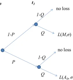
The probability that the client does not fulfill the margin requirement at t=0 is denoted by P which is supposed to be an increasing function of 𝑀 − 𝐴0. In the case of non-payment, the clearinghouse liquidates the client’s position at the closing price of the next day 𝐹1. The clearinghouse can suffer a loss in t=1 if the balance of the margin account is negative, and the client refuses to pay it with a probability of Q, which can happen both on the upward and the downward branch of the event tree presented in Figure 1.
5
Figure 1: The event tree of the loss generating process
As we can see in Figure 1, the client has limited liability, i.e. cannot be forced to pay more than he has on his account. For the sake of simplicity, we suppose that Q=1, thus the client is supposed to refuse to pay the negative balance at t=1 with certainty. For a general Q we obtain similar but much more complicated formulas; however, there are no significant changes in the key findings.
If the client does not pay the margin at t=0, we are on the downward branch of the tree and the account balance of the client at t=0 is 𝐴0. Otherwise, if the client pays the margin, we are in the upward branch of the tree and the account balance at t=0 becomes M. Once the actual account balance is determined, the loss of the CCP depends only on ∆𝐹. Therefore, we investigate the conditional expected loss for a general value of A instead of 𝑀 or 𝐴0.
Theorem 1 (Conditional expected loss of the CCP)
Under Assumptions 1-3, the conditional expected value of the loss 𝐿(𝐴) is 𝐿(𝐴) = 𝐿(𝐴, 𝜎) = 𝜎 ∙ 𝜑 (𝐴
𝜎) − 𝐴 ∙ 𝜙 (−𝐴
𝜎) (2)
where 𝜑 is the density function, and 𝜙 is the distribution function of the standard normal distribution.
Proof
𝐿(𝐴) = 𝐿(𝐴, 𝜎) = − ∫ 1
√2𝜋𝜎
0
−∞
∙ 𝑒−(𝑥−𝐴)
2
2𝜎2 𝑥 𝑑𝑥 = 𝜎 ∙ 𝜑 (𝐴
𝜎) − 𝐴 ∙ 𝜙 (−𝐴
𝜎) (3) □ no loss
no loss L(M,σ)
L(A0,σ) P
1-P
Q 1-Q 1-Q
Q
t0 t1
6
Corollary 1
The loss 𝐿(𝐴) of the CCP is a differentiable, strictly decreasing and strictly convex function of the customer’s account balance A, and
𝐴→∞lim𝐿(𝐴) = lim
𝐴→∞𝐿′(𝐴) = 0. (4)
Proof
Using equation 𝜑′(𝑥) = −𝑥 ∙ 𝜑(𝑥), we obtain 𝐿′(𝐴) = −𝜙 (−𝐴
𝜎) = 𝜙 (𝐴
𝜎) − 1. (5)
Hence, lim
𝐴→∞𝐿′(𝐴) = lim
𝑦→∞𝜙(𝑦) − 1 = 0.
Also, 𝐿′(𝐴) < 0 implies that 𝐿(𝐴) is strictly decreasing.
Further,
𝐿′′(𝐴) =𝜑 (𝐴
𝜎𝜎)> 0 (6)
which proves strict convexity.
Finally,
𝐴→∞𝑙𝑖𝑚𝐿(𝐴) = 𝑙𝑖𝑚
𝐴→∞(𝜎 ∙ 𝜑 (𝐴
𝜎) − 𝐴 ∙ 𝜙 (−𝐴 𝜎)) =
= 𝑙𝑖𝑚
𝐴→∞
𝜙 (−𝐴 𝜎)
−1 𝐴
= 𝑙𝑖𝑚
𝐴→∞
𝜑 (−𝐴 1 𝜎) 𝐴2
= 𝑙𝑖𝑚
𝐴→∞𝐴2∙ 𝜑 (𝐴 𝜎) = 0
□
Definition 1 (Unconditional expected loss of the CCP)
The unconditional expected loss 𝑈𝐿 of the CCP is calculated at t=0. According to Assumption 3, the CCP can request an extra payment at t=0, which can be refused by the client with probability 𝑃 = 𝑃(𝑀 − 𝐴0). If the requirement is fulfilled, the new account balance is 𝑀.
Otherwise it is 𝐴0. This means that the unconditional expected loss of the CCP at t=0 is 𝑈𝐿(𝐴0, 𝑀, 𝜎) = 𝑃(𝑀 − 𝐴0) ∙ 𝐿(𝐴0, 𝜎) + (1 − 𝑃(𝑀 − 𝐴0)) ∙ 𝐿(𝑀, 𝜎). (7)
7
Definition 2 (Optimal margin)
In Equation (7), 𝐴0 is exogenously given, and M is to be determined by the CCP; hence it can be considered as the control variable. The optimization problem of the CCP is to set M at an optimal level to minimize its unconditional expected loss UL.
Assumption 4 (Probability of non-payment)
We specify the probability of non-payment as
𝑃(𝑀 − 𝐴0) = 𝑃(𝑀 − 𝐴0, 𝜆) = {1 − 𝑒−𝜆∙(𝑀−𝐴0) 𝑓𝑜𝑟 𝑀 ≥ 𝐴0
0 𝑓𝑜𝑟 𝑀 < 𝐴0 (8) In Equation (8), 𝜆 is a positive parameter characterizing the overall funding (il)liquidity conditions in the economy where higher 𝜆 indicates less funding liquidity available. According to Assumption 4, the probability of non-payment is an increasing function of two symmetric factors, the overall funding illiquidity (𝜆) which determines the ability-to-pay and the payment burden (𝑀 − 𝐴0) which determines the willingness-to-pay.
Theorem 2 (Characterization of the optimal margin)
There is a unique optimal margin M satisfying
ℎ(𝑀) = 𝜆 ∙ (𝐿(𝐴0) − 𝐿(𝑀)) + 𝐿′(𝑀) = 0. (9) Proof
Obviously, 𝑀 < 𝐴0 cannot be optimal; hence we consider when M is in the interval [𝐴0,∞).
We have to minimize UL with respect to M. Its derivative in (𝐴0, ∞) and its right-derivative in 𝐴0 is
𝜕𝑈𝐿
𝜕𝑀 (𝐴0, 𝑀) = 𝜆𝑒−𝜆∙(𝑀−𝐴0)∙ (𝐿(𝐴0) − 𝐿(𝑀)) + 𝑒−𝜆∙(𝑀−𝐴0)∙ 𝐿′(𝑀) =
= 𝑒−𝜆∙(𝑀−𝐴0)∙ ℎ(𝑀)
(10)
Here we have ℎ(𝐴0) < 0 (hence UL cannot be minimal in 𝑀 = 𝐴0), and lim
𝑀→∞ℎ(𝑀) = 𝜆 ∙ 𝐿(𝐴0) > 0. As (5) and (6) imply that 𝐿(𝑀) is decreasing and 𝐿′(𝑀) is increasing; therefore ℎ(𝑀) is (continuous and) strictly increasing, so there is exactly one M satisfying ℎ(𝑀) = 0, and here ℎ changes sign from negative to positive. Multiplying this with 𝑒−𝜆∙(𝑀−𝐴0)> 0 does not change this behavior, so this is the unique optimum.□
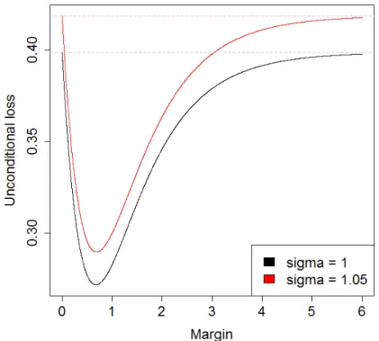
Figure 2 depicts the unconditional loss depending on the margin if 𝐴0 = 0 and 𝜆 = 1.
8
Figure 2: Unconditional loss of the clearinghouse in function of the margin requirement
We can see in Figure 2 that the loss is not a monotone function of the margin and as Theorem 2 states, there is a unique optimum. If 𝑀 goes to infinity, it is clear that lim
𝑀→∞𝑈𝐿(𝐴0, 𝑀) = 𝐿(𝐴0). No matter how large margin the CCP requests if it is not paid. The result will be the same when no margin is requested.
Definition 3 (Risk-sensitive margin)
The margin setting mechanism is weakly (strongly) risk-sensitive if the margin is a non- decreasing (increasing and linear) function of the expected volatility σ.
We note that margin systems directly linked to Value-at-Risk calculations assuming the normal distribution of log returns are strongly risk-sensitive.
Theorem 3 (Sensitivity of the optimum) The optimal margin M
(i) is a strictly increasing function of 𝐴0 and a strictly decreasing function of λ, and (ii) is not risk-sensitive even in a weak sense as its relation to 𝜎 depends on the
parameters: M is strictly increasing in 𝜎 iff 𝑒𝑀
2−𝐴02
2𝜎2 < 1 + 𝑀 𝜆𝜎2
(11)
which holds if M is sufficiently close to 𝐴0 and 𝜆 is sufficiently small.
9
Proof
Using the law of implicit derivation in formula (9) we compute 𝜕𝐴𝜕𝑀
0, 𝜕𝑀𝜕𝜆, and 𝜕𝑀𝜕𝜎. For this, we need to compute first 𝜕𝑀 𝜕ℎ, 𝜕𝐴𝜕ℎ
0, 𝜕ℎ𝜕𝜆, and 𝜕𝜎𝜕ℎ.
𝜕ℎ
𝜕𝑀 = 𝜆 (1 − 𝛷 (𝑀
𝜎)) + 𝜑 (𝑀 𝜎)1
𝜎> 0 (12)
𝜕ℎ
𝜕𝐴0 = 𝜆 (𝛷 (𝐴0
𝜎) − 1) < 0 (13)
𝜕ℎ
𝜕𝜆 = 𝐿(𝐴0) − 𝐿(𝑀) > 0 (14)
𝜕ℎ
𝜕𝜎 = 𝜆 (𝜑 (𝐴0
𝜎) − 𝜑 (𝑀
𝜎)) − 𝜑 (𝑀 𝜎)𝑀
𝜎2
(15)
The sign in (14) comes from Corollary 1 since 𝑀 > 𝐴0 in the optimum.
By (12), (13), (14), and (15), we obtain
𝜕𝑀
𝜕𝐴0 = −
𝜕𝐴𝜕ℎ0
𝜕𝑀 𝜕ℎ
> 0 (16)
𝜕𝑀
𝜕𝜆 = −
𝜕𝜆 𝜕ℎ
𝜕𝑀 𝜕ℎ
< 0 (17)
𝜕𝑀
𝜕𝜎 = −
𝜕𝜎 𝜕ℎ
𝜕𝑀 𝜕ℎ
(18)
It is clear from (16) and (17) that the optimal M is a strictly increasing function of 𝐴0 and a strictly decreasing function of 𝜆.
M is strictly increasing in 𝜎 iff 𝜕𝜎 𝜕ℎ < 0 by (12), (15), and (18) which is equivalent to (11).□
In this simplified model, we derived an intuitive result that supports the idea of anti-cyclical margin even from the point of view of the micro-level financial stability of the CCP. As we can see, the optimal margin is the function of at least three exogenous parameters: the actual account balance of the client 𝐴0, the overall funding illiquidity 𝜆, and the expected volatility 𝜎. The principle of weak risk-sensitivity would require M to be a non-decreasing function of 𝜎.
However, even in this simple model, the optimal M does not necessarily satisfy it since other
10
factors interact, as well. For example, in the case of a crisis, the client’s actual account balance can be very low, even negative due to a recent shock (low 𝐴0), and the client may have difficulties to get financing (high 𝜆). In this situation, the CCP should set a less aggressive margin far below the value-at-risk level which depends purely on the expected volatility 𝜎.
Formula (11) can be interpreted as in the optimum the CCP does not adjust the margin to the expected volatility mechanically but also considers the payment burden 𝑀 − 𝐴0 and the funding illiquidity 𝜆 which determine the client’s willingness and ability to pay, respectively. It is remarkable that the CCP should operate an anti-cyclical margin strategy merely to avoid larger losses also for its own sake without considering macro-level consequences (price impact, systemic risk, etc.) emphasized by the regulator.
Of course, margin setting is a much more complicated task in the real world than in our one- period model. First of all, there are more clients, more assets, more maturities, and more periods. The margins of today influence the accounts of tomorrow, hence the margins of tomorrow and so on. This spillover effect makes the margin setting a complex dynamic and stochastic optimization problem. Moreover, we only modeled the long side of a transaction, while in practice CCPs have to manage the long and the short sides simultaneously. And last but not least, there can be other risk factors influencing the probability and the magnitude of the losses, as well. In the next section, we perform a more realistic agent-based simulation of a hypothetical clearinghouse where we incorporate four risk factors (VIX-index, S&P100, equity market spread, and the LIBOR-OIS spread). To investigate the optimal margin setting strategy in this context, we define four margin setting methods and compare them regarding the loss distribution of the CCP.
11
3. MICROSIMULATIONS
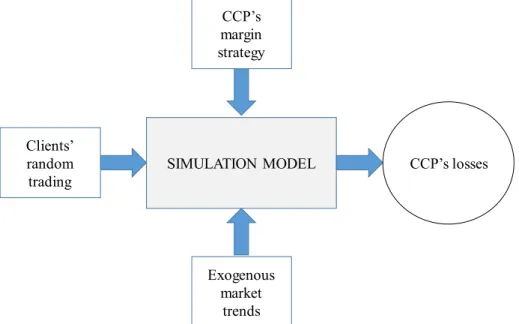
We also developed a multi-period simulation model7 of a hypothetical clearinghouse’s operation to analyze the effects of more complex margin-setting strategies. The structure of the simulation model is presented in Figure 3.
Figure 3: The structure of the simulation model
As we can see, the output of the model is the loss distribution of the CCP which depends on the exposures resulting from the client’s random trading, the margin setting strategy applied by the CCP (i.e. the control variable), and some exogenous market factors.
3.1 THE MODEL
In the following, we introduce the assumptions of the simulation model and the rationale behind them.
Assumption 5 (Futures market)
The clearinghouse is active only on the futures market of one asset, namely of the S&P100 index representing the largest caps. The two expirations take place at the next two Decembers denoted by 𝑇𝑘 where k =1 or 2. For the sake of simplicity, interest rates are supposed to be zero;
therefore, futures prices are equal to the spot prices.
7 The model can be considered as an improved and extended version of (Berlinger et al., 2016).
SIMULATION MODEL CCP’s
margin strategy
Clients’
random trading
CCP’s losses
Exogenous market
trends
12
Assumption 6 (No price impact)
Prices are independent of the trading activity of the CCP and its clients. In other words, prices are exogenously given, and players are price takers. Clients are supposed to trade at the closing price of the given day.
Assumption 6 can be justified if the market served by the clearinghouse is only a small segment of the global market.
Assumption 7 (Uninformed trading)
The number of potential clients belonging to the clearinghouse is N which is set to 300 in our simulation. Clients are uninformed and trade randomly. A trade is made between client i (long side) and client j (short side), where i, j =1,…N and i≠j. Pairs i, j are selected randomly, and all traders have equal chance to be selected. The expiration date of the trade can be 𝑇1 or 𝑇2. The probability of the first delivery date is 𝑝𝑡 which is an increasing function of the time remaining until 𝑇1(as a consequence, 1-𝑝𝑡 is the probability of the second delivery date).
𝑝𝑡= time remaining until 𝑇1
365 (19)
Assumption 7 is a technical tool to ensure continuous trading and realistic positions evolving over the 8-year-long period.
Assumption 8 (Number of trades)
The total number of trades within a day (𝐷𝑡) is a stochastic variable and comes from a binomial distribution, the expected value of which depends on the volatility of the market measured by the VIX index. The binomial distribution has the following parameters:
𝐷𝑡 = 𝐵𝑖𝑛𝑜𝑚(𝑁; 𝑝𝑡= 0.1 ∙𝑉𝐼𝑋𝑉𝐼𝑋𝑡
𝑎𝑣𝑒𝑟𝑎𝑔𝑒) (20)
where VIXaverage is the average of daily VIX-index values of the last year. To model trade numbers, the use of a binomial distribution is reasonable if we consider M clients who trade with the same probability within a day. The parameters of the distribution in (20) could be calibrated to the characteristics of a real clearinghouse.
Assumption 9 (Trade amounts)
The trade amount in the d-th trade (d =1,…,𝐷𝑡) on day t in the market at delivery date k (i.e. the number of units involved in a given trade) 𝑅𝑡,𝑑𝑘 also follows a binomial distribution depending on the market volatility.
𝑅𝑡,𝑑𝑘 = 𝐵𝑖𝑛𝑜𝑚(1000; 𝑝𝑡= 0.05 ∙𝑉𝐼𝑋𝑉𝐼𝑋𝑡
𝑎𝑣𝑒𝑟𝑎𝑔𝑒) (21)
13
The distribution of trading volume is not exhibiting “fat tail” characteristics as traders try to avoid extreme large trades by splitting their orders into smaller units to minimize the price impact. They also try to avoid very small trades because of the fixed transactional costs (Lo and Wang, 2009); therefore, we used a binomial distribution.
It is notable that Assumptions 8 and 9 make the operation of the clearinghouse pro-cyclical as clients tend to maintain larger open positions when the expected volatility is high, i.e. in crisis times.
Assumption 10 (Clients’ exposure)
The position P of the n-th client in the given trade is measured in the unit of the asset, and it is positive (negative) if the client is on the long (short) side:
𝑃𝑡,𝑑𝑛,𝑘 = {
𝑅𝑡,𝑑𝑘 if 𝑛 = 𝑖 −𝑅𝑡,𝑑𝑘 if 𝑛 = 𝑗 0 otherwise
(22)
Having simulated 𝐷𝑡 trades of different attributes within day t, we determine the net accumulated exposure (𝐸) of the n-th trader on day t, for delivery date k as
𝐸𝑡𝑛,𝑘 = 𝐸𝑡−1𝑛,𝑘 + ∑𝐷𝑑=1𝑡 𝑃𝑡,𝑑𝑛,𝑘 (23)
𝐸0𝑛,𝑘 = 0
which is also measured in the unit of the asset. According to Assumption 10, positions of opposite sign get canceled as long and short positions offset each other at a client level.
The total exposure of the clearinghouse at the end of day t is
𝐸𝑡 = ∑2𝑘=1∑𝑁𝑛=1|𝐸𝑡𝑛,𝑘| (24)
Thus, at aggregate level long and short positions do not offset each other as the clearinghouse has to manage both sides simultaneously.
Assumption 11 (Clients’ margin account)
If the n-th client fulfills the margin requirement M on day t-1, then its margin account A on day t will equal to the margin plus the result of the daily settlement:
𝐴𝑛𝑡 = {
𝑀𝑡−1𝑛 + ∑ 𝐸𝑡𝑛,𝑘∙ (𝐹𝑡𝑘− 𝐹𝑡−1𝑘 ) if long
2
𝑘=1
𝑀𝑡−1𝑛 + ∑ 𝐸𝑡𝑛,𝑘∙ (−𝐹𝑡𝑘+ 𝐹𝑡−1𝑘 )
2
𝑘=1
if short
(25)
14
Otherwise, its position will be liquidated, and the margin account in liquidation AL will be
𝐴𝐿𝑛𝑡 = {
𝐴𝑡−1𝑛 + ∑ 𝐸𝑡𝑛,𝑘∙ (𝐹𝑡𝑘− 𝐹𝑡−1𝑘 ) if long
2
𝑘=1
𝐴𝑡−1𝑛 + ∑ 𝐸𝑡𝑛,𝑘∙ (−𝐹𝑡𝑘+ 𝐹𝑡−1𝑘 )
2
𝑘=1
if short
(26)
It follows from (25) that clients immediately take off all the profits accumulated on their account. Note the similarities and differences between (1) and (25)-(26).
Assumption 12 (Margin requirement)
The margin requirement M of the n-th trader is calculated at the end of the t-th day and is valid for the next day. It is based on the liquidity adjusted value-at-risk (LaVaR) of its total portfolio 𝐸𝑡𝑛, where the significance level is 99%, the data window is w =1 year, the holding period is τ
=2 days, and s𝑡 refers to the bid-ask spread on the stock market.
𝑀𝑡𝑛 = 𝐿𝑎𝑉𝑎𝑅(𝐸𝑡𝑛, 𝑤,τ, s𝑡) ∙ 𝛽𝑡=
= raw margin ∙ buffer multiplier (27)
where 1 ≤ 𝛽𝑡≤ 1.258 is the anti-cyclical buffer multiplier which is the control variable representing the strategy of the clearinghouse. The VaR of the portfolio is calculated using a delta-normal approach, and the LaVaR is calculated from the VaR and the bid-ask spread according to Angelidis and Benos (2006):
𝐿𝑎𝑉𝑎𝑅 = 𝑉𝑎𝑅 +s2𝑡𝐸𝑡𝑛 (28)
Of course, LaVaR is higher if in the last one-year period the volatility was higher and the actual market liquidity is lower (i.e. the bid-ask spread is higher). The applied buffer multiplier 𝛽𝑡 modifies the raw margin, determines the margin requirement, and depends purely on the clearinghouse’s strategy.
The total margin requirement set by the clearinghouse at the end of the t-th day is
𝑀𝑡 = ∑𝑁𝑛=1𝑀𝑡𝑛 (29)
In reality, if several clearinghouses compete for the clients a lower level of average margin can be a competitive advantage. However, we exclude this effect, and in our model, the margin level is critical for the clearinghouse because of its effect on the loss distribution.9
8 The range for the anti-cyclical buffer variable comes from the EMIR Supplementing Regulation No. 153/2013, Article 28, a) cited in the introduction.
9 This was true also in the one-period model.
15
Assumption 13 (Probability of non-payment)
Clients are supposed to fulfill the initial margin requirement always. Later on, if the margin account of client n is less than the requirement, 𝑀𝑡𝑛 > 𝐴𝑡𝑛, the clearinghouse sends a margin call to the client requiring to pay the difference. It is possible that the client does not want to or cannot pay. Exactly like in (8), the probability of non-payment P is an increasing function of two factors: the payment burden 𝑀𝑡𝑛− 𝐴𝑡𝑛 (willingness-to-pay) and the funding illiquidity 𝜆𝑡 (ability-to-pay), the latter is being represented by the OIS-Libor spread in this simulation model.
According to Assumptions 12 and 13, a higher margin increases the coverage of the position provided the client pays, however, at the same time, it also increases the probability of non- payment. These two effects have impacts of opposite sign on the loss of the clearinghouse, which constitutes a fundamental trade-off the clearinghouse has to deal with.
Assumption 14 (Conditional loss of the CCP)
In the case of non-payment, the client's position is liquidated at the next day's closing price, which can cause losses to the CCP. The loss of the clearinghouse L on the t-th day is defined as the sum of the losses on each client whose position is in liquidation according to (30), i.e. the sum of the margin accounts in liquidation AL with a negative balance:
𝐿𝑡 = ∑𝑁𝑛=1𝐿𝑛𝑡 = ∑𝑁𝑛=1(𝐴𝐿𝑛𝑡)− = −∑𝑁𝑛=1𝑚𝑖𝑛(𝐴𝐿𝑛𝑡; 0) (30) According to Assumptions 5, 8, 9, 11, 12, 13, and 14, market factors have nontrivial effects on the losses of the CCP as summarized in Table 1.
Table 1: The effects of market factors on the CCP’s losses
Factor Content Direct effect Model variable
S&P index spot price futures price F
S&P index historical volatility margin requirement M
VIX index volatility expectations trading volume E
bid-ask spread market illiquidity margin requirement M LIBOR-OIS funding illiquidity probability of default P
The S&P index has a direct effect on the clients’ account due to the daily settlement, but its historical evolution also has an indirect effect on the raw margin through the LaVaR calculation.
The interference of these four market factors also considered as crisis proxies will influence the loss of the clearinghouse in a complex way, which can be captured by the simulation.
16
Assumption 15 (Margin strategies)
We define four margining strategies to determine the value of the control parameter 𝛽𝑡 in formula (27).
1. Full smoothing: the margin requirement is the raw margin that is βt is equal to 1, and the raw margin is calculated as a fixed percentage (≈21%) of the actual value of the position.10
2. No smoothing: a constant margin buffer is applied under any circumstances: βt is constant (≈1.09) over time.11
3. Immediate transition: under normal market circumstances the margin buffer is 25%
(βt=1.25), while in a crisis the buffer is released immediately (βt=1).12
4. Smooth transition: βt ranges between 1 and 1.25 and a smooth transition is ensured by limiting the change of the margin relative to the previous day by the formula:13
𝑀𝑡𝑛 = 𝑚𝑎𝑥[𝑚𝑖𝑛[𝑀𝑡−1; 𝐿𝑎𝑉𝑎𝑅(𝐸𝑡𝑛, 𝑤,τ, s𝑡) ∙ 1.25]; 𝐿𝑎𝑉𝑎𝑅(𝐸𝑡𝑛, 𝑤,τ, s𝑡)] (31) The full smoothing strategy (1) is a naïve methodology which also corresponds to option (c) of anti-cyclical strategy offered by the EMIR. In the no smoothing strategy (2) anti-cyclicality concerns are not taken into consideration at all, which corresponds to the situation before the latest regulatory changes. The strategy of immediate transition (3) sense necessitates determining whether we are in a crisis or not, and right at the beginning of a crisis, the margin buffer is immediately released; while at the end of the crisis, the buffer is immediately rebuilt.
It is not risk-sensitive even in the weak sense. Contrary to this, in the case of the strategy of smooth transition (4), the process of releasing and rebuilding the buffer is slowed down by formula (31). Both strategies (3) and (4) are consistent with option (a) of anti-cyclical margin setting mechanism recommended by the EMIR. According to Definition 3, Strategies (1) and (3) are not risk-sensitive even in the weak sense, strategy (2) is strongly risk-sensitive, and strategy (4) is only weakly risk-sensitive.
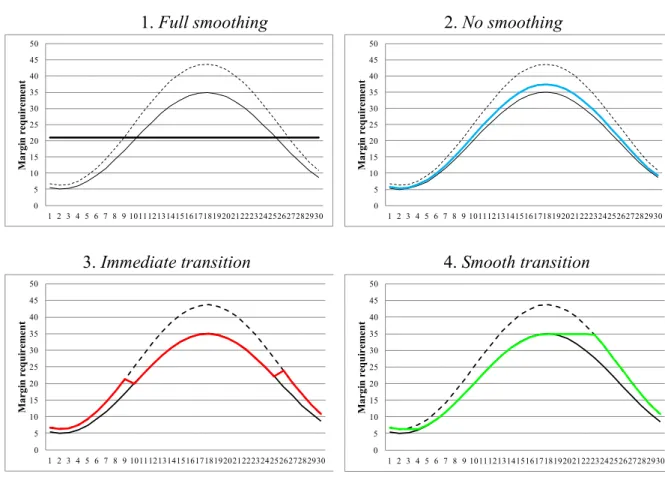
Figure 4 illustrates the above-described margin strategies assuming a stylized 30-day crisis which is manifested in the temporary increase of the calculated LaVaR driven by the volatility and the market spread. The continuous black line indicates the raw margin (the actual LaVaR), the dotted line is the raw margin multiplied by 1.25 (margin with the maximal buffer), and the colored thicker line is the applied margin requirement (M).
10 The fixed percentage is calibrated in a way that the average level of the margin over the whole period be approximately the same for all the four strategies.
11 The buffer multiplier is calibrated in a way that the average level of the margin over the whole period be approximately the same for all the four strategies.
12 The crisis periods could be determined by a stress indicator presented in (Berlinger et al. 2016), however, to avoid model calibration issues to interfere, here we defined crisis periods exogenously relying on experts’ opinion.
13 This is similar to the methodology proposed by Béli and Váradi (2017).
17
Figure 4: Illustration of the four investigated margin strategies
1. Full smoothing 2. No smoothing
3. Immediate transition 4. Smooth transition
We selected these margin strategies to represent the most relevant practices recommended by the previous and the actual regulations. They cover a complete spectrum from strong risk- sensitivity (no smoothing) to full anti-cyclicality (full smoothing). Other possible anti-cyclical strategies can be found in (Murphy et al. 2016).
In the next section, we analyze the effects of these margin strategies in terms of the resulting loss distribution of the hypothetical clearinghouse.
3.2 RESULTS AND DISCUSSION
We simulated 100 different paths14 for the clearinghouse in the 8-year-long period15 from the beginning of 2008 until the end of 2015. For each path and for each day, we calculated the total margin requirement 𝑀𝑡 (29) and the total loss of the clearinghouse 𝐿𝑡 (30) and divided these amounts by the number of open contracts 𝐸𝑡 (24), i.e. the total exposure of the clearinghouse.
Then, we averaged these ratios (𝑀𝐸𝑡
𝑡 and 𝐿𝐸𝑡
𝑡) across the 100 realized paths for each day.
Figure 5 presents how the average margin/exposure evolved between 2008 and 2015 depending on the margin strategies.
14 These paths were very similar to each other; thus, there was no need to increase the number of trajectories.
15 Time series were 9-year-long, but we used a time window of 1 year for the LaVaR calculation, therefore, we simulated the realized losses only for eight years.
0 5 10 15 20 25 30 35 40 45 50
1 2 3 4 5 6 7 8 9 101112131415161718192021222324252627282930
Margin requirement
0 5 10 15 20 25 30 35 40 45 50
1 2 3 4 5 6 7 8 9 101112131415161718192021222324252627282930
Margin requirement
0 5 10 15 20 25 30 35 40 45 50
1 2 3 4 5 6 7 8 9 101112131415161718192021222324252627282930
Margin requirement
0 5 10 15 20 25 30 35 40 45 50
1 2 3 4 5 6 7 8 9 101112131415161718192021222324252627282930
Margin requirement
18
Figure 5: Margin/exposure under different margin strategies, 2008-2015 (USD/number of open position)
Based on Figure 5, we can formulate Result 1.
Result 1 (Risk-sensitivity of the strategies)
Strategies of immediate transition and smooth transition correlate positively to the no smoothing strategy representing the principle of strict risk-sensitivity. The full smoothing strategy represents the principle of anti-cyclicality in an extreme way and correlates negatively to the other three.
We can observe in Figure 5 that the margin under the full smoothing strategy (black line) moves contrary to the other three: it declines in the crisis and increases afterward. As the margin is always a fixed percentage of the portfolio value, essentially, the changes in the margin requirements reflects the changes in the position value. Hence, the full smoothing strategy can be considered as the least risk-sensitive and the most anti-cyclical one. The opposite is the no smoothing strategy (blue line) which is the utmost risk-sensitive. The immediate transition strategy (red line) switches sharply between the regimes of crisis and no crisis determined by the stress indicator, while the smooth transition strategy produces more stable but still weakly risk-sensitive margin requirements. Both of them relates more closely to the no smoothing strategy as it is also reflected in the pairwise correlation coefficients, presented in Table 2.
19
Table 2: Pairwise correlation between margin requirements under different margin strategies, 2008-2015
1. Full smoothing
2. No smoothing
3. Immediate transition
4. Smooth transition
1. Full smoothing 1.00 -0.47 -0.42 -0.55
2. No smoothing 1.00 0.96 0.95
3. Immediate transition 1.00 0.93
4. Smooth transition 1.00
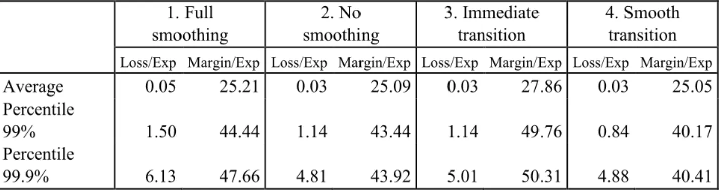
To assess which margin strategy is the most beneficial for the clearinghouse, we can compare the corresponding loss distributions in terms of their average and their tail percentiles (99% and 99.9%) for the investigated period, see Table 3.
Table 3: Average loss and loss percentiles under different margin strategies, 2008-2015
1. Full smoothing
2. No smoothing
3. Immediate transition
4. Smooth transition Loss/Exp Margin/Exp Loss/Exp Margin/Exp Loss/Exp Margin/Exp Loss/Exp Margin/Exp
Average 0.05 25.21 0.03 25.09 0.03 27.86 0.03 25.05
Percentile
99% 1.50 44.44 1.14 43.44 1.14 49.76 0.84 40.17
Percentile
99.9% 6.13 47.66 4.81 43.92 5.01 50.31 4.88 40.41
According to Table 3, the average margin level of the strategies are approximately the same, but it is the smooth transition strategy which requires the lowest level of average margin (25.05) while its average loss and loss percentiles are also relatively low. However, the no smoothing strategy has somewhat lower loss percentile at 99.9% level. Therefore, these characteristics in themselves are insufficient to assess the relative attractiveness of the strategies. We can compare the loss distributions in a systematic way by examining whether there exists a first or a second order stochastic dominance between them.
Result 2 (First-order stochastic dominance)
On this sample, the full smoothing strategy is first-order stochastically dominated by all the three other strategies.
The first order dominance can be judged by observing the function 𝐹(𝑥) for each strategy which we get by cumulating the observed loss/exposure frequencies 𝑝(𝑦) for all 𝑦 ≥ 𝑥:
𝐹(𝑥) = ∑+∞𝑦=𝑥𝑝(𝑦) (32)
Lower values of 𝐹(𝑥) are more favorable for the clearinghouse, see Figure 6.
20
Figure 6: The comparison of margin strategies with first order stochastic dominance of loss distribution under different margin strategies, 2008-2015
According to Result 2, a rational clearinghouse would not choose the full smoothing strategy if it expects the future market conditions to be similar to the past ones.
We can compare the strategies with the help of the second order dominance, as well.
Result 3 (Second-order stochastic dominance)
On this sample, the immediate transition strategy is second-order stochastically dominated by both no smoothing and smooth transition strategies. However, these latter two strategies are not dominating each other. (Of course, the full smoothing strategy is also second-order stochastically dominated by all the others.)
The second order dominance can be judged by observing the function 𝑇(𝑥) for each strategy which we get by cumulating the values 𝐹(𝑦) for all 𝑦 ≥ 𝑥:
𝑇(𝑥) = ∑+∞𝑦=𝑥𝐹(𝑦) (33) and as before, lower 𝑇(𝑥) values are more favorable for the clearinghouse, see Figure 7. 16
16 As expected, functions 𝑇(𝑥) are smoother than functions 𝐹(𝑥).
0 2 4 6
Cumulated probability F(x)
Loss/Exposure
1. Full smoothing 2. No smoothing 3. Immediate transition 4. Smooth transition
21
Figure 7: The comparison of margin strategies with second order stochastic dominance of loss distribution under different margin strategies, 2008-2015
This means that a risk-averse clearinghouse will prefer no smoothing and smooth transition strategies to the immediate transition strategy – at least if market factors are expected to behave stationary over time. The dominance of no smoothing and smooth transition strategies is even more convincing if we consider that their average margin levels (25.09 and 25.05 respectively) are lower than that of immediate transition strategy (27.86), see Table 3.
Finally, we also examined the relative performance of the margin setting strategies in different crises. The investigated period 2008-2015 contains five significant stress events of different characteristics: Lehman-fall, flash-crash, EU sovereign debt crisis, Russian crash, and Chinese crash.
Result 4 (Relative crisis performance)
The bad overall relative performance of the full smoothing strategy was due to the longstanding and deep crisis right after the Lehman-fall. In the other four less significant crises the most anti- cyclical full smoothing strategy would have been the optimal one as it cost the least to the clearinghouse, see Figure 8 and Table 4.
0 2 4 6
Repeatedly cumulated probability T(x)
Loss/Exposure
1. Full smoothing 2. No smoothing 3. Immediate transition
4. Smooth transition
22
Figure 8: Losses over time under different strategies (loss/exposure)
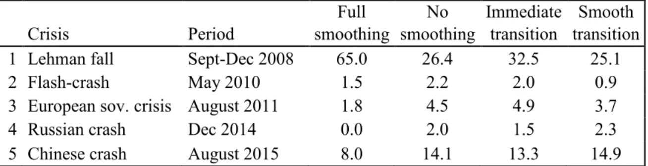
Summing up the losses within each crisis period, we can calculate the total cost of the crisis to the clearinghouse, at least in this narrow sense, see Table 4.
Table 4: The total cost of the largest crises to the hypothetical clearinghouse
Crisis Period
Full smoothing
No smoothing
Immediate transition
Smooth transition
1 Lehman fall Sept-Dec 2008 65.0 26.4 32.5 25.1
2 Flash-crash May 2010 1.5 2.2 2.0 0.9
3 European sov. crisis August 2011 1.8 4.5 4.9 3.7
4 Russian crash Dec 2014 0.0 2.0 1.5 2.3
5 Chinese crash August 2015 8.0 14.1 13.3 14.9
As Table 4 shows, the most expensive crisis was that of the Lehman-fall when the full smoothing strategy would have caused the highest losses by far. However, in the other less significant crises, the full smoothing strategy would have performed much better than the other strategies (except flash crash where the smooth transition strategy performed slightly better).
This is consistent with our findings in the one-period model: in the case of a prolonged crisis with longstanding and increasing volatility, a moderated, “anti-cyclical" margin setting strategy fails to reflect the increasing risk; hence the coverage of the positions becomes insufficient leading to increased losses. But, in minor and temporary crises, anti-cyclical smoothing strategies help both the clients and the clearing house to survive at a relatively low cost.
Concerning the two dominating strategies, it is notable that in 2008-2011 (Lehman-fall, flash- crash, European sovereign crisis) the smooth transition strategy performed somewhat better, while recently (Russian crash and Chinese crash) it was the no smoothing strategy which cost slightly less. We can conclude, therefore, that the selection of the margin strategy depends heavily on what kind of crises we expect to come.
0 1 2 3 4 5 6 7
Oct-07 Oct-08 Oct-09 Oct-10 Oct-11 Oct-12 Oct-13 Oct-14 Oct-15
1. Full smoothing 2. No smoothing 3. Immediate transition 4. Smooth transition
23
4. CONCLUSIONS
In this paper, we compared different margin strategies in terms of their effects on the loss distribution of the clearinghouse assuming that its activity has no impact on the market prices.
First, in the framework of a simple, one-period model we examined the fundamental trade-off between the confronting requirements of risk-sensitivity and anti-cyclicality. We proved that a well-chosen margin strategy could create significant value for the clearinghouse. The optimal strategy is non-trivial; in most cases, it lies inside the set of feasible strategies and represents a delicate compromise between different forces. The optimal margin is higher if the actual balance of the client is higher if clients are supposed to get financing easily (i.e. funding illiquidity is low), but its relation to the expected volatility can be positive or negative depending on the other factors. It follows that a strongly risk-sensitive strategy is not always optimal for the clearinghouse; hence, the need for anti-cyclical margin setting can be justified not only at the macro level (by the regulator) but also at the micro level (by the interests of the clearinghouse itself).
We also performed a more realistic agent-based simulation of a hypothetical clearinghouse active on the US stock market where we incorporated several crisis proxies (VIX-index, S&P100, equity market spread, and the LIBOR-OIS spread). We defined four margin strategies (full smoothing, no smoothing, immediate transition, and smooth transition) and found that full smoothing strategy was first-order stochastically dominated by all the other three strategies;
therefore, a rational player would refuse it. However, it is notable that this underperformance was solely due to the Lehman-fall while in the other crises this strategy cost surprisingly less than the others did. We also found that the anticyclical strategy based on immediate transition was second-order stochastically dominated by both the classical no smoothing and the freshly propagated smooth transition strategies. Although the strategy of immediate transition is consistent with the prescription of the regulation, a risk-averse clearinghouse should avoid it.
It was hard to differentiate between the two dominating strategies, as their risk profiles were very similar. In 2008-2011 (Lehman-fall, flash-crash, European sovereign crisis) the smooth transition strategy performed somewhat better, while recently (Russian crash and Chinese crash) it was the no smoothing strategy which cost slightly less.
We can conclude that margin-smoothing strategies serve not only macro-level (regulatory) interests, but also clearinghouses can reduce their direct losses coming from the liquidation of the positions with the help of anti-cyclical margin strategies. This is particularly the case when the actual high volatility is considered only temporary. Therefore, it is a critical issue for clearinghouses to forecast future volatility trends effectively.
ACKNOWLEDGEMENT
This research was supported by the scholarship of Bolyai János of the Hungarian Academy of Sciences. We would also like to thank the participants of the 2016 Annual Financial Market Conference for their valuable comments.
24
REFERENCES
1. Angelidis, T., Benos, A. 2006. Liquidity-adjusted Value-at-risk Based on the Components of the Bid-ask Spread. Applied Financial Economics, 16(11), 835-851.
2. Barker, R., Dickinson, A., Lipton, A., Virmani, R. 2016. Systemic Risks in CCP Networks. arXiv preprint arXiv:1604.00254.
3. Béli, M., Váradi, K. 2017. A Possible Methodology of Defining Initial Margin.
Financial and Economic Review, forthcoming
4. Berlinger, E., Dömötör, B., Illés, F., Váradi, K. 2016. Stress Indicator for Clearing Houses. Central European Business Review, 5(4), 47-60.
5. Brunnermeier, M. K., Pedersen, L. H. 2009. Market Liquidity and Funding Liquidity. Review of Financial Studies, 22(6), 2201-2238.
6. Cont, R., Kokholm, T. 2014. Central Clearing of OTC Derivatives: Bilateral vs.
Multilateral Netting. Statistics & Risk Modeling, 31(1), 3-22.
7. Commission Delegated Regulation (EU) No 153/2013 of 19 December 2012, supplementing Regulation (EU) No 648/2012 of the European Parliament and of the Council with regard to regulatory technical standards on requirements for central counterparties.
http://eur-lex.europa.eu/LexUriServ/LexUriServ.do?uri=OJ:L:2013:052:0041:0074:EN:PDF Accessed: 8th September 2015.
8. Danielsson, J., Embrechts, P., Goodhart, C., Keating, C., Muennich, F., Renault, O., Shin, H. S. 2001. An Academic Response to Basel II. Special Paper-LSE Financial Markets Group.
9. Danielsson, J., Shin, H. S., Zigrand, J. P. 2011. Endogenous and Systemic Risk. Risk Research, http://riskresearch.org/files/DanielssonShinZigrand2013.pdf, Accessed: 20th April 2016.
10. Day, T. E., & Lewis, C. M. 2004. Margin Adequacy and Standards: An Analysis of the Crude Oil Futures Market. The Journal of Business, 77(1), 101-135.
11. Domanski, D., Gambacorta, L., Picillo, C. 2015. Central clearing: trends and current issues. BIS Quarterly Review December.
12. Duffie, D., Scheicher, M., Vuillemey, G. 2015. Central Clearing and Collateral Demand. Journal of Financial Economics, 116(2), 237-256.
13. European Market Infrastructure Regulation: Regulation (EU) No 648/2012 of the European Parliament and of the Council of 4 July 2012, on OTC derivatives, central counterparties and trade repositories.
http://eur-lex.europa.eu/LexUriServ/LexUriServ.do?uri=OJ:L:2012:201:0001:0059:EN:PDF Accessed: 8th September 2015.
14.
Financial Stability Board 2016. OTC Derivatives Market Reforms Eleventh Progress Report on Implementation, August15. Fenn, G. W., Kupiec, P. 1993. Prudential Margin Policy in a Futures‐ style Settlement System. Journal of Futures Markets, 13(4), 389-408.
16. Figlewski, S. 1984. Margins and Market Integrity: Margin Setting for Stock Index Futures and Options. Journal of Futures Markets, 4(3), 385-416.
17. Glasserman, P., Wu, Q. 2017. Persistence and Pro-cyclicality in Margin Requirements.
Columbia Business School Research Paper No. 17-34. Available at SSRN: https://ssrn.com/abstract=2938515
25
18. Heath, A., Kelly, G., Manning, M., Markose, S., Shaghaghi, A. R. 2016. CCPs and Network Stability in OTC Derivatives Markets. Journal of Financial Stability, 27, 217- 233.
19. Heller, D., Vause, N. 2012. Collateral Requirements for Mandatory Central Clearing of Over-the-counter Derivatives. BIS Working Paper No. 373.
20. Kiff, J., Elliott, M. J. A., Kazarian, E. G., Scarlata, J. G., Spackman, C. 2009. Credit Derivatives: Systemic Risks and Policy Options? (No. 9-254). International Monetary Fund.
21. Kiff, J., Dodd, R., Gullo, A., Kazarian, E., Lustgarten, I., Sampic, C., & Singh, M. 2010.
Making Over-the-Counter Derivatives Safer: The Role of Central Counterparties. Global Financial Stability Report.
22. Lo, A. W., Wang, J. 2009. Stock Market Trading Volume. in Y. Ait-Sahalia and L.
Hansen, eds., The Handbook of Financial Econometrics. New York: North-Holland.
23. Murphy, D., Vasios, M., Vause, N. 2014. An Investigation into the Pro-cyclicality of Risk-based Initial Margin Models. Bank of England Financial Stability Paper No. 28.
24. Murphy, D., Vasios, M., Vause, N. 2016. A Comparative Analysis of Tools to Limit the Pro-cyclicality of Initial Margin Requirements. Staff working paper No. 597, Bank of England
25. O’Donoghue, C. 2001. Dynamic Microsimulation: A Methodological Survey. Brazilian Electronic Journal of Economics, 4(2), 77.
26. Wooldridge, P. 2016. Central Clearing Predominates in OTC Interest Rate Derivatives Markets. BIS Quarterly Review, 22-4.