Infectious Disease Modelling

(1)

Modeling the impact of quarantine during an outbreak of Ebola virus disease

Attila D enes

^a^,^*

, Abba B. Gumel

^b^,¹

aBolyai Institute, University of Szeged, Aradi vertanúk tere 1., Szeged H-6720, Hungary

bSchool of Mathematical and Statistical Sciences, Arizona State University, Tempe, AZ 85287-1804, USA

a r t i c l e i n f o

Article history:

Received 22 October 2018

Received in revised form 20 January 2019 Accepted 27 January 2019

Available online 5 February 2019 Handling Editor: J Wu

Keywords:

Ebola virus disease Quarantine Global dynamics

a b s t r a c t

The quarantine of people suspected of being exposed to an infectious agent is one of the most basic public health measure that has historically been used to combat the spread of communicable diseases in human communities. This study presents a new deterministic model for assessing the population-level impact of the quarantine of individuals suspected of being exposed to disease on the spread of the 2014e2015 outbreaks of Ebola viral disease. It is assumed that quarantine is imperfect (i.e., individuals can acquire infection during quarantine). In the absence of quarantine, the model is shown to exhibit global dynamics with respect to the disease-free and its unique endemic equilibrium when a certain epidemiological threshold (denoted byR0) is either less than or greater than unity.

Thus, unlike the full model with imperfect quarantine (which is known to exhibit the phenomenon of backward bifurcation), the version of the model with no quarantine does not undergo a backward bifurcation. Using data relevant to the 2014e2015 Ebola transmission dynamics in the three West African countries (Guinea, Liberia and Sierra Leone), uncertainty analysis of the model show that, although the current level and effectiveness of quarantine can lead to signiﬁcant reduction in disease burden, they fail to bring the associatedquarantine reproduction number (R^Q₀) to a value less than unity (which is needed to make effective disease control or elimination feasible). This reduction ofR^Q₀is, however, very possible with a modest increase in quarantine rate and effectiveness. It is further shown,viasensitivity analysis, that the parameters related to the effectiveness of quarantine (namely the parameter associated with the reduction in infectiousness of infected quarantined individuals and the contact rate during quarantine) are the main drivers of the disease transmission dynamics. Overall, this study shows that the singular implementation of a quarantine intervention strategy can lead to the effective control or elimination of Ebola viral disease in a community if its coverage and effectiveness levels are high enough.

©2019 The Authors. Production and hosting by Elsevier B.V. on behalf of KeAi Communications Co., Ltd. This is an open access article under the CC BY-NC-ND license (http://creativecommons.org/licenses/by-nc-nd/4.0/).

*Corresponding author.

E-mail address:denesa@math.u-szeged.hu(A. Denes).

Peer review under responsibility of KeAi Communications Co., Ltd.

1 Other afﬂiation: Department of Mathematics and Applied Mathematics, University of Pretoria, Pretoria 0002, South Africa Contents lists available atScienceDirect

Infectious Disease Modelling

j o u r n a l h o m e p a g e :w w w . k e a i p u b l i s h i n g . c o m / i d m

https://doi.org/10.1016/j.idm.2019.01.003

2468-0427/©2019 The Authors. Production and hosting by Elsevier B.V. on behalf of KeAi Communications Co., Ltd. This is an open access article under the CC BY-NC-ND license (http://creativecommons.org/licenses/by-nc-nd/4.0/).

(2)

1. Introduction

Ebola virus disease (EVD), whichﬁrst appeared in 1976 in Zaire (Bowen et al., 1977;Johnson, Webb, Lange,&Murphy, 1977), is one of the most virulent viral diseases of humans, with a case fatality ratio estimated between 25 and 90%

(World Health Organization, 2018a). EVD is transmitted between humans through contact with blood, secretions, organs or other bodilyﬂuids of infected or dead humans or animals, and its incubation period range between 2 and 21 days. The symptoms are vomiting, diarrhea, body rash, tremors and in some cases, both internal and external bleeding. The largest Ebola outbreak so far started in Guinea in December 2013 (World Health Organization, 2015). During this epidemic, almost 29,000 people contracted the disease which resulted in more than 11,000 deaths, mostly in Guinea, Liberia and Sierra Leone. A new outbreak started recently (on 4 April 2018) in the Democratic Republic of the Congo and (as of October 20, 2018) there have already been 237 Ebola cases and 153 deaths (World Health Organization, 2018b).

Quarantine, deﬁned loosely as the temporary removal (from their immediate abode or the general population) of people suspected of being exposed to a communicable disease, has historically been used as an effective basic public health control measure to prevent the spread of infectious diseases. There are numerous issues pertaining to the logistic of the actual implementation of quarantine as a control strategy, such as who should be quarantined and for how long suspected people should be in quarantine (these have major socio-economic and public health implications). For instance, in the case of the 2014 outbreaks of the EVD, some US states imposed a three-week quarantine period for all health care workers who returned to the United States from the Ebola-affected regions (where they may have cared for patients with Ebola) (Campbell, Adan,&

Morgado, 2017;Drazen et al., 2014). It was, however, shown by Haas (Haas, 2014) that the three-week period may not be optimal (in particular, it was shown that exposed individuals with 0.2%e12% risk of developing disease may be released from quarantine prior to the end of the incubation period). On August 1, 2014, the three Western African countries affected by the epidemic (Guinea, Liberia and Sierra Leone) announced the enforcement of a mass quarantine in vast forest areas around their common borders that are considered the epicentre of the outbreak (a few days later, Liberian authorities imposed a 10-day quarantine over West Point; Sierra Leone announced, on September 6, a nationwide mass quarantine between September 19 and 21) (Eba, 2014).

Numerous mathematical modeling studies have been conducted to study the transmission dynamics and control of EVD.

In fact, the earliest mathematical models for EVD appeared long before the 2014e15 epidemic. Chowell et al. (Chowell, Hengartner, Castillo-Chavez, Fenimore,&Hyman, 2004) proposed a stochastic SEIR model toﬁt data from the 1995 and 2000 outbreaks in Congo and Uganda. This model was further developed by Legrand et al. (Legrand, Grais, Boelle, Valleron,&

Flahault, 2007) by including two new compartments for hospitalized people and for people who died from Ebola but have not yet been buried. Several new models appeared soon after the start of the 2014 outbreak (Nishiura&Chowell, 2014;Towers, Patterson-Lomba,&Castillo-Chavez, 2014). The model by Legrand et al. was used to study the 2014e15 Ebola outbreaks by Rivers et al. (Rivers, Lofgren, Marathe, Eubank,&Lewis, 2014). Webb and Browne incorporated age of infection in their model (Webb&Browne, 2016). Tsanou et al. considered the role of host-reservoir transmission (with bats as reservoir) of EVD and spillover potential to humans (Tsanou, Bowong, Lubuma,&Mbang, 2017). Furthermore, Tsanou et al. (Tsanou, Lubuma, Ouemba Tasse, &Tenkam, 2018) studied the impact of environmental contamination on the transmission dynamics of EVD. Several other studies incorporated the effect of anti-EVD control measures, such as increasing hospitalization, timely burial of people who died from EVD and distribution and use of protective kits in households (Althaus, 2014;Barbarossa et al., 2015;Lewnard et al., 2014). For instance, Agusto et al. (Agusto, Teboh-Ewungkem,&Gumel, 2015) studied the effect of traditional beliefs and customs on the transmission dynamics of the disease.

A number of mathematical models, typically of the form of deterministic systems of nonlinear differential equations, have been designed and used to gain insight into the population-level impact of quarantine (of people suspected of being exposed to a disease) and isolation (of people with clinical symptoms of a communicable disease) on the spread and control of infectious diseases (see, for instance, the models in (Day, Park, Madras, Gumel,&Wu, 2006;Gumel et al., 2004;Hethcote, Zhien,

&Shengbing, 2002;Lipsitch et al., 2003;Mubayi, Kribs Zaleta, Martcheva,&Castillo-Chavez, 2010;Nu~no, Feng, Martcheva,&

Castillo-Chavez, 2005;Safi&Gumel, 2010;Safi&Gumel, 2013;Safi&Gumel, 2015;Yan&Zou, 2008)). Hethcote (Hethcote et al., 2002) presented SIQS (susceptible-infected-quarantined-susceptible) and SIQR (susceptible-infected-quarantined- recovered) models for the dynamics of an infectious disease that is controllable using quarantine and isolation, showing that the use of quarantine-adjusted incidence induces the phenomenon of Hopf bifurcation in the transmission dynamics of the disease.Nu~no et al. (2005)also showed oscillatory dynamics in an SIQR model for the dynamics of two strains of influenza in a population. Similarly, a probabilistic model was designed and used by Day et al. (Day et al., 2006) to determine the conditions under which quarantine is expected to be useful. The Day et al. study showed that the number of infections averted through quarantine is expected to be low if isolation is effective, but the number increases abruptly as the effectiveness of isolation diminishes. It is worth mentioning, however, that in majority of the quarantine, or quarantine and isolation, models in the literature (including the models in all of the aforementioned studies, with exception of those in (Lipsitch et al., 2003;Mubayi et al., 2010;Safi&Gumel, 2013)), the term“quarantine”was generally incorrectly used to refer to the removal of individuals who already have been infected with the disease (either in the exposed/latent (Day et al., 2006;Gumel et al., 2004;Safi&

Gumel, 2010;Saﬁ&Gumel, 2015), or even in the symptomatic (Hethcote et al., 2002;Nu~no et al., 2005) class). In other words, the term“quarantine”was used instead of the more epidemiologically-appropriate term,“isolation”. As stated earlier, quarantine is the temporary removal of susceptible individuals who are feared to have been exposed to a communicable

enes, A.B. Gumel / Infectious Disease Modelling 4 (2019) 12e27

(3)

disease. These (currently-susceptible-but-feared-exposed) individuals are temporarily removed from the actively-mixing population until, at the very least, after the incubation period of the disease, after which they are tested to determine whether or not they have the disease. If they have acquired the infection, they are then placed in isolation. If they do not show clinical symptoms of the disease at the end of the quarantine period, they return to the susceptible (and actively-mixing) population. People can be quarantined at home (i.e., self-quarantine) or in public health facility (such as hospital, health centers or makeshift facility, such as the military tents used during the 2014 ebola outbreaks (Drazen et al., 2014)). Quarantine is correctly modeled in a few studies, including in (Lipsitch et al., 2003;Mubayi et al., 2010;Safi&Gumel, 2013). In particular, Lipsitch et al. (Lipsitch et al., 2003) modeled quarantine of susceptible individuals based on the number of individuals with clinical symptoms of the disease in the community. In addition to allowing for the quarantine of susceptible individuals, the model developed by Safiand Gumel (Safi&Gumel, 2013) also accounted for the adjustment of the disease incidence function to account for the actively-mixing population (in line with Hethcote (Hethcote et al., 2002)). These features were also incorporated in the model developed by Mubayi et al. (Mubayi et al., 2010). It is worth stating, however, that the quarantine models in (Lipsitch et al., 2003;Mubayi et al., 2010) do not allow breakthrough infection during quarantine. In other words, the models in (Lipsitch et al., 2003;Mubayi et al., 2010) assume perfect quarantine (this assumption is relaxed in the current study).

The purpose of the current study is to design a new model for realistically assessing the population-level impact of quarantine (assumed to be imperfect, so that individuals in quarantine can acquire infection during quarantine) on the spread and control of the 2014e2015 EVD outbreaks in the three affected Western African countries. The paper is organized as follows. The model is formulated andﬁtted with observed data in Section2(the basic properties of the model, as well as the local asymptotic stability result for the associated disease-free equilibrium, are also given). A special case of the model, in the absence of quarantine, is rigorously analysed in Section3. Numerical simulations of the full model are reported in Section5.

2. Formulation of mathematical model

The model is formulated as follows. The total population at timet, denoted byNðtÞ, is split into the population of those in quarantine (denoted byN_QðtÞ) and those not in quarantine (denoted byN_UðtÞÞ, so thatNðtÞ ¼ N_QðtÞ þ N_UðtÞ. The total population of individuals in quarantine at timetis divided into those that are susceptibleðS_QðtÞÞ, exposed (E_QðtÞ; that is, infected but not yet infectious) and symptomaticðI_QðtÞÞ. Hence,

N_QðtÞ ¼S_QðtÞ þE_QðtÞ þI_QðtÞ:

Similarly, the total population of individuals not in quarantine at timetis sub-divided into the sub-populations of susceptible (S_UðtÞ), exposed (E_UðtÞ), symptomatic (I_UðtÞ), treatedðI_TðtÞÞ, recoveredðRðtÞÞ, deadðDðtÞÞ, so that

N_UðtÞ ¼S_UðtÞ þE_UðtÞ þI_UðtÞ þI_TðtÞ þRðtÞ þDðtÞ:

Theforce of infectionassociated with the model to be developed (denoted bylðtÞ) is given by

l

^{ðtÞ ¼}^I^U^{ðtÞ þ}

h

TI_TðtÞ þ

h

QI_QðtÞ þ

h

DDðtÞ

N_UðtÞ ; (1)

wherehT,hQandhDare modiﬁcation parameters accounting for the variability of the infectiousness of infected individuals in theI_T,I_Q andDclasses, in comparison to those in theI_U class, respectively. Following Lipsitch et al. (Lipsitch et al., 2003), quarantine is modeled as follows: a fraction,q, of susceptible individuals who are feared exposed to Ebola (i.e., by having contact with a conﬁrmed Ebola case) are placed in quarantine. Owing to its assumed imperfect nature, individuals in quarantine can be infected (and moved to the compartmentE_Q) with probabilityb(quarantined individuals remain susceptible and stay in the quarantined susceptibleS_Q class during quarantine with probability 1b). Quarantined individuals who do not develop the disease at the end of the quarantine period are moved to theS_Uclass at a rater_Q.

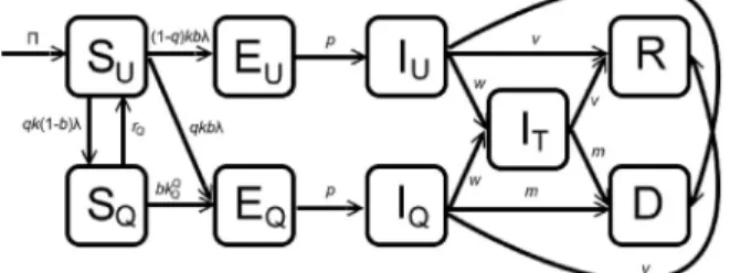
Fig. 1.Flow diagram of the model (2).

(4)

The model is given by the following deterministic system of nonlinear differential equations (where a prime denotes differentiation with respect to timet; a schematic diagram of the model is depicted inFig. 1and the parameters of the model are described inTable 1):

S⁰_UðtÞ ¼

P

^kbSUðtÞ

l

^ðtÞ^qkð1^bÞSUðtÞ

l

^{ðtÞ þ}^rQS_QðtÞ dS_UðtÞ;

S⁰_QðtÞ ¼qkð1bÞS_UðtÞ

l

^ðtÞ^bk

Q

QS_QðtÞI_QðtÞ

N_QðtÞ r_QS_QðtÞ dS_QðtÞ;

E⁰_UðtÞ ¼ ð1qÞkbS_UðtÞ

l

^ðtÞ^pEUðtÞ dE_UðtÞ;

E⁰_QðtÞ ¼qkbS_UðtÞ

l

^{ðtÞ þ}^bk

Q

QS_QðtÞI_QðtÞ

N_QðtÞ pE_QðtÞ dE_QðtÞ;

I⁰_UðtÞ ¼pE_UðtÞ ðvþmþwÞI_UðtÞ dI_UðtÞ;

I⁰_ΤðtÞ ¼w

I_UðtÞ þI_QðtÞ

ðvþmÞI_TðtÞ dI_TðtÞ;

I⁰_QðtÞ ¼pE_QðtÞ ðvþmþwÞI_QðtÞ dI_QðtÞ;

R⁰ðtÞ ¼v

I_UðtÞ þI_TðtÞ þI_QðtÞ dRðtÞ;

D⁰ðtÞ ¼m

I_UðtÞ þI_TðtÞ þI_QðtÞ fDðtÞ;

(2)

with the auxiliary equation

B⁰ðtÞ ¼fDðtÞ;

andl^ðtÞas given by (1). In (2),Pis the recruitment rate (by birth or immigration),kis the average daily per capita contact rate in the community, bis the transmission probabilitypercontact (here, we follow Lipsitch et al. (Lipsitch et al., 2003) in separating the parameterskandbinstead of applying the usual composite transmission parameterb. That is, we assume that each infectious individual makeskcontactsperday, and a proportion,b, of these contacts lead to infection). The parametersq anddrepresent, respectively, the quarantine rate of susceptible individuals and the natural mortality rate (the latter rate is assumed to be the same in all epidemiological compartments). Individuals in quarantine acquire EVD infection at a ratebk^Q_Q. The parameterpaccounts for the rate of progression from any of the exposed classes (E_U orE_Q) to the corresponding symptomatic class (IUorI_Q). That is, 1=pis the mean incubation period of the disease. Infectious individuals in theIUandI_Q classes are hospitalized at a ratew. The parametersvandmare, respectively, the recovery rate and per capita disease-induced

Table 1

Description, ranges and baseline values of parameters of the model (2).

Parameter Description Baseline value

(range)

Ref.

P Recruitment rate 11826/week World Health Organization (2018c)

d Natural death rate 0.00054/week World Health Organization (2018c)

b Transmission probability per contact 0.054 Legrand et al. (2007)

hT Modiﬁcation parameter for infectiousness of hospitalized individuals

0.86 Legrand et al. (2007)

hQ Modiﬁcation parameter for infectiousness of infected quarantined individuals

0.502 (0.5e0.9) Legrand et al. (2007) hD Modiﬁcation parameter for infectiousness of Ebola-deceased

individuals

3.89 Legrand et al. (2007)

k Average per capita contact rate in the community 9.15/week Legrand et al. (2007) q Quarantine rate of susceptible individuals 0.125 (0.05e0.5)/

week

Fitted

rQ Rate of release from quarantine 1.107 (0.5e2)/

week

Fitted

k^Q_Q Average per capita contact rate during quarantine 7.97/week Fitted

1=p Incubation period 1.498 week (Gomes et al., 2014;Legrand et al., 2007;Pandey

et al., 2014)

v Recovery rate 0.362/week (Gomes et al., 2014;Legrand et al., 2007)

m Ebola-induced death rate 0.797/week (Gomes et al., 2014;Legrand et al., 2007;Pandey

et al., 2014)

w Hospitalization rate 1.58/week (Gomes et al., 2014;Legrand et al., 2007;Rivers

et al., 2014)

1=f Mean time from death due to Ebola to burial 0.762 weeks World Health Organization (2015) enes, A.B. Gumel / Infectious Disease Modelling 4 (2019) 12e27

(5)

death rate. Ebola-deceased individuals are buried at a ratef(i.e., 1=fis the mean time from death to burial for Ebola-deceased individuals) (Agusto et al., 2015;Barbarossa et al., 2015;Legrand et al., 2007). It is worth emphasizing that, in contrast to Lipsitch et al. (Lipsitch et al., 2003), it is assumed in this study that hospitalized individuals can transmit infection (hence, the mean duration of infectiousness is 1=ðwþmþvÞ).

The model (2) is an extension of many existing models for quarantine and isolation (such as those in (Gumel et al., 2004;

Hethcote et al., 2002;Lipsitch et al., 2003;Mubayi et al., 2010;Nu~no et al., 2005;Safi&Gumel, 2010;Safi&Gumel, 2013;Safi

&Gumel, 2015;Yan&Zou, 2008)) by,inter alia:

1. Incorporating the quarantine of susceptible individuals (this was not included in the models in (Gumel et al., 2004;

Hethcote et al., 2002;Nu~no et al., 2005;Saﬁ&Gumel, 2010;Saﬁ&Gumel, 2015;Yan&Zou, 2008)).

2. Using nonlinear quarantine rate of susceptible individuals (linear rates were used in (Mubayi et al., 2010;Saﬁ&Gumel, 2013)).

3. Allowing for breakthrough infection during quarantine (perfect quarantine and isolation were assumed in (Lipsitch et al., 2003;Mubayi et al., 2010). That is, the models in (Lipsitch et al., 2003;Mubayi et al., 2010) assume that susceptible individuals in quarantine do not acquire infection during the quarantine period).

4. Allowing for disease transmission by infected individuals in quarantine and/or isolation (this was not accounted for in the models in (Lipsitch et al., 2003;Mubayi et al., 2010)).

5. Allowing for the heterogeneity between infected individuals in quarantine and isolation and those not in quarantine and isolation (i.e., we stratify the infected population intoEQ andIQ for those in quarantine and isolation, andEUandIUfor those not in quarantine and isolation). This allows for the assessment of the effectiveness of an intervention strategy aimed at encouraging infected people in quarantine and isolation to positively modify their behavior so that they do not continue to generate more infections (this stratiﬁcation is not considered in the model in (Mubayi et al., 2010). That is, all infected individuals are lumped into the same compartment in (Mubayi et al., 2010), regardless of their quarantine or isolation status).

Further, the model (2) extends many of the EVD models in the literature (such as those in (Agusto et al., 2015;Chowell et al., 2004;Tsanou et al., 2017)) by,inter alia, allowing for the quarantine of susceptible individuals and disease acquisition and transmission during quarantine and isolation (or hospitalization).

2.1. Basic qualitative properties

The basic qualitative properties of the model (2), with respect to the nonnegativity and boundedness of solutions, will now be explored.

Lemma 2.1. Suppose that the initial values S_Uð0Þ, S_Qð0Þ, E_Uð0Þ, E_Qð0Þ, I_Uð0Þ, I_Tð0Þ, I_Qð0Þ, Rð0Þ, Dð0Þ, Bð0Þof the model (2) are all nonnegative. Then, the solution of (2) starting with these initial values will remain nonnegative for all time t>0. Furthermore, all solutions of the model (2) are bounded.

Proof.The proof for the nonnegativity component of the theorem is by contradiction (see Theorem A4 of (Thieme, 2003)).

Suppose that the statement of the lemma (with respect to nonnegativity) does not hold. That is, there is at least one of the nine state variables of the model (2), and at ¼t0, such that the value of this state variable goes through 0 att ¼t, and all state variables of the model take nonnegative values for 0tt. For example, consider the state variable isS_UðtÞ. It can be seen that the derivative ofS_UðtÞis positive ifS_UðtÞ ¼0. Hence,S_UðtÞcannot decrease further once it has reached 0. The case of each of the other state variable of the model can be shown in a similar way.

To show that all solutions of the model (2) are bounded, it is convenient to deﬁneN ðtÞ ¼S_UðtÞ þS_QðtÞ þE_UðtÞ þE_QðtÞ þ I_UðtÞ þI_TðtÞ þI_QðtÞ þRðtÞ þDðtÞandd^¼^minff;dg. Thus,

N⁰ðtÞ ¼

P

^d^SUðtÞ þS_QðtÞ þE_UðtÞ þE_QðtÞ þI_UðtÞ þI_TðtÞ þI_QðtÞ þRðtÞ fDðtÞ

P

d

NðtÞ;

from which it follows that lim sup_t_/∞NðtÞ ^P_d. Using the fact that all solutions are nonnegative, the second statement of the lemma is established.∎

Deﬁne the following feasible region for the model (2):

G

^¼^SUðtÞ;S_QðtÞ;E_UðtÞ;E_QðtÞ;I_UðtÞ;I_TðtÞ;I_QðtÞ;RðtÞ;DðtÞ

2ℝ⁹þ:NðtÞ

P d

:

The result below follows from the above analyses.

Lemma 2.2. The regionGis positively-invariant for the model (2) for every nonnegative initial condition inℝ⁹þ. enes, A.B. Gumel / Infectious Disease Modelling 4 (2019) 12e27

(6)

2.2. Dataﬁtting

It should,first of all, be stated that good estimates for pretty much all the non-quarantine related parameters of the model (2) are available in the literature, as tabulated inTable 1. Further, good estimates for one of the four quarantine-related parameters (hQ) are available. Thus, our task is tofind good estimates for the remaining three quarantine-related parameters of the model (k^Q_Q,rQ andq). In order to do so, and to subsequently validate the model, wefitted the model using the available cumulative data for the 2014e15 Ebola outbreaks in three affected West African countries. We apply Latin Hypercube Sampling (a Monte-Carlo sampling method used in statistics to measure simultaneous variation of several model parameters (McKay, Beckman,&Conover, 1979)) to generate a representative sample set from the parameter ranges for the three quarantine-related parameters (k^Q_Q,r_Q andq), while the baseline values for the rest of the parameters, given inTable 1, are used as well. For all elements of this representative sample set, we numerically calculate the solutions of the model (2) with the given parameter values and apply the least squares method tofind the parameters which give the bestfit. We consider the data of thefirst 40 weeks of the outbreak (World Health Organization, 2018d) (as tabulated inTable 2), as after this time, several intervention measures were implemented (hence, the estimates for many of the control-related parameters of the model, including the transmission, hospitalization and burial rates, changed significantly). The estimated values of the two quarantine-related parameters of the model obtained from thefitting exercise are tabulated inTable 1. The simulation results obtained for the cumulative number of cases, byfitting the model with the data of thefirst 40-week period, are depicted in Fig. 2. Thefigure shows a reasonably goodfit (thereby adding realism to the predictive capacity of the model (2)). The goodness of thefit is theoretically measured by computing the associatedaverage relative errorof thefit using the formula

401

P40 i¼1jyib^yij

jyij z0:8163, wherey_iandby_iare the exact and estimated cumulative number of cases for Weekiði¼1;2; /; 40Þ (depicted inTable 2), respectively. The reasonably small value of the relative error (0.8134) conﬁrms the goodness of theﬁt obtained.

Table 2

Cumulative number of cases reported (sum of conﬁrmed, suspected and probable cases) in theﬁrst forty weeks of the 2014e2015 Ebola epidemic in Western Africa (World Health Organization, 2018d).

Weeks Guinea Liberia Sierra Leone

1 1 1 1

2 5 1 1

3 9 2 1

4 13 2 1

5 21 3 2

6 23 3 2

7 28 4 3

8 35 4 3

9 39 5 4

10 44 5 4

11 47 6 5

12 103 8 6

13 127 8 6

14 158 25 6

15 203 27 12

16 218 35 12

17 226 35 12

18 236 35 12

19 248 35 12

20 248 35 12

21 291 35 50

22 344 35 81

23 351 35 89

24 398 41 136

25 398 51 158

26 413 115 252

27 413 142 337

28 413 196 442

29 427 249 525

30 472 391 574

31 495 554 717

32 519 786 810

33 607 1082 910

34 648 1378 1026

35 771 1698 1216

36 899 2407 1478

37 942 3022 1673

38 1074 3458 2021

39 1199 3834 2437

40 1350 4076 2950

(7)

3. Analysis of special case of the model: quarantine-free with mass action incidence

We consider,ﬁrst of all, a special case of the model (2) in the absence of quarantine (i.e., the model (2) withq¼0) and constant total population (i.e., the model (2) with mass action incidence, rather than standard incidence). The two assumptions are made for mathematical tractability, in addition to allowing for the determination of whether or not adding quarantine to the resulting model (without quarantine) will alter its dynamical features. The second assumption of constant total population is justiﬁed since Ebola-induced mortality is generally very negligible, in comparison to the total population in the affected areas (World Health Organization, 2018d). The quarantine-free model with constant total population is given by:

S⁰_UðtÞ ¼

P

^kbSUðtÞI_UðtÞ kb

h

TS_UðtÞI_TðtÞ kb

h

DS_UðtÞDðtÞ dS_UðtÞ;

E⁰_UðtÞ ¼kbS_UðtÞI_UðtÞ þkb

h

TS_UðtÞI_TðtÞ þkb

h

DS_UðtÞDðtÞ pE_UðtÞ dE_UðtÞ;

I⁰_UðtÞ ¼pE_UðtÞ ðvþmþwÞI_UðtÞ dI_UðtÞ;

I⁰_TðtÞ ¼wI_UðtÞ ðvþmÞI_TðtÞ dI_TðtÞ;

R⁰ðtÞ ¼v½IUðtÞ þI_TðtÞ dRðtÞ;

D⁰ðtÞ ¼m½I_UðtÞ þI_TðtÞ fDðtÞ:

(3)

The reduced model (3) has a disease-free (trivial) equilibrium (DFE),E0 ¼ ðS_U;E_U;I_U;I_T;R;DÞ ¼

Pd;0;0;0;0;0 , and a non- trivial (positive) endemic equilibrium point (EEP)

E1¼

S_U;E_U;I_U;I_T;R;D

¼

P

^ðd^þ^pÞE

d ;E; pE

dþmþvþw; pwE

ðdþmþvÞðdþmþvþwÞ; pvE

dðdþmþvÞ; mpE fðdþmþvÞ ; whereE ¼_dþp¹

1_R¹

0 , withR0(the basic reproduction number of the model (3)) given by R₀¼

P

^bkp½dðf^þ

h

DmÞ þfðmþvþ

h

TwÞ þ

h

DmðmþvþwÞ

dfðdþpÞðdþmþvÞðdþmþvþwÞ :

The non-trivial equilibriumE1exists wheneverR0>1 (it should be noted that theS_Ucomponent of this equilibrium is positive forR0>1, since 1_R¹

0<1 andP>1).

Fig. 2.Fitting the model to the data for the 2014e2015 Ebola outbreaks in Western Africa (World Health Organization, 2018d): cumulative number of new infected cases (Parameter values used are as given inTable 1).

(8)

3.1. Global asymptotic stability of equilibria 3.1.1. Disease-free equilibrium

The global asymptotic stability property of the DFE (E0) of the model (3) will be explored using the approach in [38, Theorem2.1]. It is worth recalling the following result.

Theorem A. ([ (Shuai&van den Driessche, 2013),Theorem2.1]).

Consider the system x⁰¼F ðx;yÞ V ðx;yÞ;

y⁰¼gðx;yÞ (4)

withg ¼ ðg₁;…;gmÞ^T. The vectorsx¼ ðx₁;…;xnÞ2ℝⁿ andy¼ ðy₁;…;ymÞ^T2ℝ^m represent the populations in the disease compartments and the disease-free compartments, respectively. The functionsF andV are deﬁned asF ¼ ðF 1;…;F nÞ^T andV ¼ ðV 1;…;V nÞ^Tsuch thatF idenotes the rate of new infections in theith disease compartment andVi;i¼1;…;n denote transition terms. Assume that the disease-free systemy⁰¼gð0;yÞhas a unique equilibriumy₀>0 which is locally asymptotically stable within the disease-free space. Deﬁne the twonnmatricesFandVas

F¼ vF _i vx_j ð0;y₀Þ

!

and V¼ vV _i vx_j ð0;y₀Þ

!

;

and let,

fðx;yÞ:¼ ðFVÞxF ðx;yÞ þV ðx;yÞ:

Furthermore, letu^T0 be the left eigenvector of the matrix V¹F corresponding to the eigenvalueR0. Iffðx;yÞ 0 in G3ℝ^nþmþ ,F0,V¹0 andR01, thenQ¼u^T^V¹^xis a Lyapunov function for (4) onG^.

Theorem 3.1. The disease-free equilibrium E0of the model (3) is globally-asymptotically stable inG~:¼ fðSUðtÞ;EUðtÞ;IUðtÞ;ITðtÞ; RðtÞ;DðtÞÞ2ℝ⁶_þgwheneverR01.

Proof.Using the notation inTheorem Aabove, the next generation matrices,VandF, associated with the model (3) are given, respectively, by

V¼ 0 BB

@

dþp 0 0 0

p dþmþvþw 0 0

0 w dþmþv 0

0 m m f

1 CC

A and F¼ 0 BB BB BB

@ 0 b

P

^k

d

b

P

^k

h

T

d

bBk

h

D

d

0 0 0 0

1 CC CC CC A

;

and the functionfis given by fðS_U;E_U;I_U;I_T;R;DÞ^T¼

bkð

P

^dSUÞðD

h

Dþ

h

TI_TþI_UÞ

d ;0;0;0 :

Hence, each condition ofTheorem Ais satisﬁed. Further, it follows from the above derivations thatu^T^V¹^xis a Lyapunov function for (3), whereuis the left eigenvector of the matrixV¹Fcorresponding to the eigenvalueR0. The statement of the theorem follows from LaSalle's Invariance Principle (LaSalle&Lefschetz, 1961).∎

3.1.2. Endemic equilibrium

The global asymptotic stability property of the endemic equilibriumE1of the model (3) will be explored using results from (Shuai&van den Driessche, 2013). It is worth recalling the following result.

Theorem B. ([ (Shuai&van den Driessche, 2013),Theorem3.5]).

Let U be an open set inℝⁿ.Consider a differential equation system

z⁰_k¼f_kðz₁;z₂;…;zmÞ; k¼1;2;…;m; (5)

withz¼ ðz₁;z₂;…;zmÞ2U.

Suppose the following assumptions are satisﬁed.

(9)

1. There exist functionsD_i:U/ℝ,G_ij:U/ℝand constantsa_ij0 such that for every 1in,D⁰_i¼D⁰_ij_ð5ÞPn

j¼1a_ijG_ijðzÞ forz2U.

2. ForA¼ ½a_ij, each directed cycleC of the weighted digraphG deﬁned by the weight matrixAhas P

ðs;rÞ2EðCÞ

GrsðzÞ 0 for z2U, whereEðCÞdenotes the arc set of the directed cycleC.

Then, there exist constantsc_i0 such that the functionDðzÞ ¼Pn

i¼1c_iD_iðzÞis a Lyapunov function for (5).

We claim the following result.

Theorem 3.2. The endemic equilibriumE1of the model (3) is globally-asymptotically stable in

G

~yn

ðS_UðtÞ;E_UðtÞ;I_UðtÞ;I_TðtÞ;RðtÞ;DðtÞÞ2ℝ⁶þ:E_UðtÞ ¼I_UðtÞ ¼I_TðtÞ ¼DðtÞ ¼0o

ifR0>1.

Proof.Deﬁneh:ℝ/ℝashðxÞ ¼x1lnxand letD₁ ¼h SUðtÞ

S_U þ^E_S Uh

EUðtÞ

E ,D₂ ¼h IUðtÞ

I_U ,D₃¼h ITðtÞ

I_T andD₄ ¼ h

DðtÞ

D . At the endemic equilibrium, the following equalities hold:

P

^¼^kbSUI_U þkb

h

TS_UI_T þkb

h

DS_UDþdS_U; pþd¼kbS_UI_U þkb

h

TS_UI_T þkb

h

DS_UD

E ;

vþmþwþd¼pE I_U ; vþmþd¼wI_U

I_T ; f¼mI_U þI_T

D :

Noting thathðxÞ 0 for allx>0 andhðxÞ ¼0 if and only ifx¼1, and applying the above equalities, gives:

D⁰₁ðtÞ kbI_U I_UðtÞ

I_U lnI_UðtÞ I_U E_UðtÞ

E lnE_UðtÞ E þkb

h

TI_T

I_TðtÞ

I_T lnI_TðtÞ I_T E_UðtÞ

E lnE_UðtÞ E þkb

h

DD

DðtÞ

DlnI_UðtÞ I_U E_UðtÞ

E lnE_UðtÞ E :¼a₁₂G₁₂þa₁₃G₁₃þa₁₄G₁₄; D⁰₂ðtÞ pE

I_U E_UðtÞ

E lnE_UðtÞ E I_UðtÞ

I_U lnI_UðtÞ

I_U :¼a₂₁G₂₁; D⁰₃ðtÞ wI_U

I_T I_UðtÞ

I_U lnI_UðtÞ I_U I_TðtÞ

I_T lnI_TðtÞ

I_T :¼a₃₂G₃₂; and;

D⁰₄ðtÞ mI_U D

I_UðtÞ

I_U lnI_UðtÞ I_U DðtÞ

D lnDðtÞ D þmI_T

D I_TðtÞ

I_T lnI_TðtÞ I_T DðtÞ

DlnDðtÞ D ; :¼a₄₃G₄₃þa₄₂G₄₂:

Hence, Assumption (1) ofTheorem Bholds. Deﬁne the weighted digraphðG;AÞassociated with the weight matrixA¼ ½a_ij, witha_ijdeﬁned as the constants in the above inequalities (and all othera_ij's not mentioned above are set to zero; see also Fig. 3).

For all cycles ofðG;AÞ, the Assumption (2) ofTheorem Bcan easily be veriﬁed. For instance, the case of the cycle①/②/

③/④is veriﬁed as follows. For this cycle,

(10)

G₁₄þG₄₃þG₃₂þG₂₁

¼ DðtÞ

DlnI_UðtÞ I_U E_UðtÞ

E lnE_UðtÞ

E þ

I_TðtÞ

I_T lnI_TðtÞ I_T DðtÞ

DlnDðtÞ D þ

I_UðtÞ

I_U lnI_UðtÞ I_U I_TðtÞ

I_T lnI_TðtÞ I_T þ

E_UðtÞ

E lnE_UðtÞ E I_UðtÞ

I_U lnI_UðtÞ I_U

¼0:

The other cases can be handled in a similar way. Hence, the statement of the theorem follows fromTheorem B.

It is worth stating that, using the baseline values of the parameters inTable 1, the value of the basic reproduction number (R0) isR0¼1:403>1 (hence, it follows fromTheorem 3.2that the disease will persist in the population). It is further worth noting that this value ofR0lies in the range given in numerous modeling studies for the 2014 EVD outbreaks (such as those in (Agusto et al., 2015;Barbarossa et al., 2015;Gomes et al., 2014;Nishiura&Chowell, 2014;Towers et al., 2014)).

4. Analysis of full model with quarantine and standard incidence

In this section, the local asymptotic stability of the DFE of the full model (2) (with both quarantine and standard incidence) will be analysed. The DFE of the full model is given by:

E01¼

S_U;S_Q;E_U;E_Q;I_U;I_T;I_Q;R;D

¼

P

d;0;0;0;0;0;0;0;0 ;

and it can be shown (using the next generation operator method (Diekmann, Heesterbeek, &Roberts, 2010; van den Driessche&Watmough, 2002)) that the associatedquarantine reproduction number, denoted byR^Q₀, is given by:

R^Q₀ ¼bkp

m

h

DðmþvþwþdÞ þqf

m

h

Qþv

h

Qþd

h

Qþw

h

T

þ ð1qÞfðmþvþw

h

TþdÞ

fðdþpÞðdþmþvÞðdþmþvþwÞ :

The result below follows from Theorem 2 of (van den Driessche&Watmough, 2002).

Theorem 4.1. The DFE of the full model (2),E01, is locally-asymptotically stable ifR^Q₀<1, and is unstable ifR^Q₀>1.

As in (Safiand Gumel, 2013,2015), the model (2) can be shown (using standard tools, such as the centre manifold theory (Castillo-Chavez&Song, 2004)) to undergo the phenomenon of backward bifurcation atR^Q₀ ¼1, a dynamic phenomenon associated with the co-existence of stable disease-free equilibrium and a stable endemic equilibrium when the associated reproduction threshold,R^Q₀, is less than unity. The epidemiological implication of this phenomenon, which arises due to the imperfect nature of quarantine to prevent disease transmission during quarantine (i.e., leaky quarantine), is that having R^Q₀<1, while necessary, is no longer sufficient for the effective control of the disease. In other words, quarantine-induced backward bifurcation makes the effort for the effective control of Ebola more difficult. Hence, this study shows that adding imperfect quarantine to the quarantine-free Ebola transmission model (3) induces a new dynamical phenomenon (backward bifurcation) that was not present in the quarantine-free model.

4.1. Uncertainty and sensitivity analysis

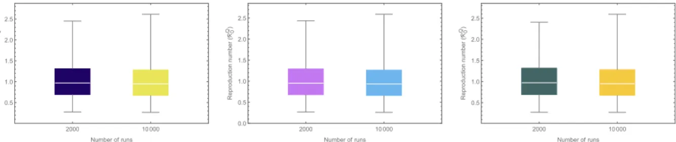
The model (2) contains numerous parameters, and uncertainties are expected to arise in the estimates of the parameter values used in the model simulations. Uncertainty analysis, using Latin Hypercube Sampling (LHS) (Blower&Dowlatabadi, 1994), is used to account for such uncertainty. The baseline values and ranges of the parameters inTable 1are used for this analysis, and it is assumed each parameter of the model obeys a uniform distribution. Using the quarantine reproduction number (R^Q0) as the response function, the results for the uncertainty analysis obtained show thatR^Q0lies in the rangeð0:268;

Fig. 3.The weighted digraphðG;AÞconstructed for model (3).

(11)

2:585Þ, with a mean 1:013>1 (Fig. 4(a)). This simulation suggests that, although the community-wide implementation of quarantine signiﬁcantly reduces the basic reproduction number (R0¼1:403 in this case), this level (and effectiveness) of quarantine is unable to lead to the effective control of the disease (sinceR^Q0 >1, albeitonly slightly). However, if the parameterhQ, for the reduction of infectiousness of quarantined-infected individuals, is further reduced from its baseline value (e.g., if it is reduced from 0.502 to 0), the mean value ofR^Q₀ reduces to 0:997<1 (so that effective disease control is feasible in this case) (seeFig. 4(b)). Similarly, increasing the quarantine rate (q) from the current baseline value ofq¼0:125 to q¼0:4, for instance, leads to a reduction of meanR^Q₀ fromR^Q₀ ¼1:009 toR^Q₀ ¼0:997 (seeFig. 4(c)). In other words, these simulations show that the singular implementation of quarantine strategy in the community can lead to the effective control (or elimination) of the disease if the coverage (q) and effectiveness of quarantine to prevent transmission during quarantine (i.e., reducehQ) is high enough.

Furthermore, sensitivity analysis is carried out, using Partial Rank Correlation Coefﬁcients (PRCCs (Blower&Dowlatabadi, 1994)), to determine the parameters of the model (2) that have the highest impact on the disease dynamics. For these simulations, the cumulative number of new cases is chosen as the response function. The sensitivity analysis based on the PRCC ranks the effect of the parameters on the response function (or outcome), while varying the parameters in their given ranges (parameters with higher positive (negative) PRCC values are positively (negatively) correlated with the response function).Table 3depicts the resulting PRCC values obtained for the parameters of the model, from which it follows that the average contact rate in the communityðkÞand the probability of transmission per contact (b) are the most dominant parameters that affect the response function (the cumulative number of cases). The mean length of time for the burial of Ebola- deceased individuals (1=f) is also shown to be inﬂuential, as expected (having the third highest PRCC value in magnitude).

Further, of the quarantine-related parameters, those related to the quarantine of susceptible individuals (q) and the reduction of the infectiousness of quarantined-infected individuals (h^QQ) are also influential (albeitwith significantly decreased PRCC values in magnitude in comparison to the PRCC values ofkandb). Thus, this study suggests that a quarantine program that significantly decreases the value ofh^Q_Q(which can be achieved by effectively treating infected quarantined individuals and/or limiting their contacts with susceptible individuals during quarantine) or increaseq(by increasing the contact tracing and quarantining of people feared exposed to EVD infection) can lead to a significant reduction in disease burden.

Fig. 4.Box plot of the reproduction number (R^Q₀) with 2000, resp. 10000 LHS runs. Parameter values used are as given inTable 1.

Table 3

Partial rank correlation coefﬁcients of parameters of model 2.

Parameter Description PRCC

b Transmission probabilitypercontact 0.72

k Average per capita contact rate in the community 0.78

q Quarantine rate of susceptible individuals 0.23

hT Modiﬁcation parameter for infectiousness of hospitalized individuals 0.18

hQ Modiﬁcation parameter for infectiousness of infected quarantined individuals 0.19

hD Modiﬁcation parameter for infectiousness of Ebola-deceased individuals 0.35

1=rQ Length of stay in quarantine 0.23

k^Q_Q Average per capita contact rate during quarantine 0.19

1=p Incubation period 0.22

v Recovery rate 0.08

m Ebola-induced death rate 0.39

w Hospitalization rate 0.24

1=f Mean time from death due to Ebola to burial 0.43

(12)

5. Numerical simulations

Further numerical simulations are carried out to assess the population-level impact of the quarantine-related parameters of the model (2). These simulations show, in particular, that while the quarantine of susceptible individuals (q) and the average duration in quarantine (1=r_Q) have marginal impact on the cumulative number of new Ebola cases (Figs. 5 and 6, respectively), the modification parameter for transmission during quarantine (hQ) and the contact rate during quarantine (k^Q_Q) have significant impact on the disease burden (Figs. 7 and 8, respectively). In other words, these simulations show that the parameters related to the efficacy of quarantine (hQ andk^Q_Q) play a more significant role on the disease dynamics than the parameters related to quarantine rate of susceptible individuals (q) and length of quarantine (r_Q). A contour plot of the quarantine reproduction number (R^Q₀), as a function ofhQandq, is depicted inFig. 9, from which it follows thatR^Q₀ decreases with decreasing values ofhQ and increasing values ofq. Hence, this plot further supports the earlier result that the implementation of a quarantine strategy that reduces the infectiousness of quarantined-infected individuals (coupled with increased quarantine rate,q) will result in significant reduction of disease burden in the community.

6. Discussion and conclusion

Quarantine of individuals suspected of being exposed to a contagious disease is one of the oldest public health measures for combatting the spread of such contagious diseases in populations. This study presents a new deterministic model for

Fig. 5.Effect of quarantine of susceptible individuals (q) on the number of new Ebola cases. Parameter values used are as given inTable 1, with different values of q.

Fig. 6.Effect of duration of quarantine (1=rQ) on the cumulative number of new Ebola cases. Parameter values used are as given inTable 1, withrQ¼0:33;rQ¼ 1:54 (ﬁtted value) andrQ ¼3.

(13)

assessing the population-level impact of the implementation of quarantine on the control of the 2014 Ebola outbreaks in West Africa. The model wasfitted using data relevant to the EVD dynamics in Guinea, Liberia and Sierra Leone. Some of the notable features of the model include the explicit modeling of quarantine of both susceptible and infected individuals (in line with the approach by Lipsitch et al. (Lipsitch et al., 2003)) and the assumption that quarantine is imperfect (so that disease transmission can occur during quarantine). Detailed theoretical analysis of a special case of the model, in the absence of quarantine and with constant total population, was carried out. The analysis revealed that the disease-free equilibrium of the resulting quarantine-free model is globally-asymptotically stable whenever a certain epidemiological quantity (the basic reproduction number of the model, denoted byR0) is less than unity. The epidemiological implication of this result is that, in the absence of quarantine, bringingR0to a value less than unity is necessary and sufficient for the effective control of the disease in the population. The quarantine-free model is also shown to have a unique endemic equilibrium (where Ebola persists in the population), which is globally-asymptotically stable, wheneverR0>1. The full model with quarantine was also analysed, from which it was deduced that adding imperfect quarantine to the quarantine-free model introduces a dynamic phenomenon (backward bifurcation) that was not present in the former model. Thus, the community-wide implementation of imperfect quarantine measures (except if implemented with high efficacy to minimize disease transmission during quarantine) may fail to lead to the effective control of the disease. The presence of backward bifurcation in the transmission dynamics of a disease makes its effective control more difficult (since a lot more effort is needed to reduce the associated reproduction number further below unity, outside the backward bifurcation region).

Detailed uncertainty and sensitivity analysis are carried out on the parameters of the model to assess the impact of uncertainties in the estimates of parameter values (on the numerical simulation results obtained) and determine the parameters that are most influential to the disease transmission dynamics (as measured in terms of the cumulative number of new infections). It was shown that while the current level and efficacy of quarantine significantly reduces the value of the basic reproduction number (R0) of the model (hence, significantly reduces disease burden), it fails to bring this number to a value less than one (so that disease elimination is feasible). However, a modest increase in quarantine rate and/or the effectiveness level of quarantine (with respect to either reduction in the infectiousness of quarantined-infected individuals (hQ) or Fig. 7.Effect of modification parameter for disease transmission during quarantine (hQ) on the cumulative number of new Ebola cases. Parameter values used are as given inTable 2, withhQ¼0:05;hQ¼0:502 (fitted value),hQ¼0:75 andhQ ¼1.

Fig. 8.The effect of the per capita contact rate (k^Q_Q) during quarantine.

(14)

minimizing contact during quarantineðk^Q_QÞ) can reduce the quarantine reproduction number of the model (R^Q0) to a value less than one (thereby making effective disease control or elimination feasible).

The results of the sensitivity analysis carried out show that the contact rate in the community (k), transmission probability per contact (b) and the mean duration before burying Ebola-deceased individuals (1=f) have the most inﬂuence on the disease burden (as measured in terms of the cumulative number of new cases). Thus, these simulation results suggest that control measures that decrease the impact of these parameters (e.g., minimizing contacts with people suspected of the disease or reducing the time before an Ebola-deceased individual is buried) will be quite effective in minimizing disease burden. Our results suggest that the quarantine of susceptible individuals and the average duration in quarantine have a smaller effect on the number of infected, the modiﬁed transmission rate during quarantine and the contact rate for quarantined people have an important effect on the spread of the disease. The results of this study show that the prospects of the effective control of EVD using quarantine alone are bright, provided the coverage and effectiveness levels are high enough.

Declaration of conﬂict of interest

The authors declare no conﬂict of interest.

Acknowledgements

A. Denes was supported by the Janos Bolyai Research Scholarship of the Hungarian Academy of Sciences, by the project no.

128363, implemented with the support provided from the National Research, Development and Innovation Fund of Hungary, ﬁnanced under the PD_18 funding scheme and by the project no. 125628, implemented with the support provided from the National Research, Development and Innovation Fund of Hungary,ﬁnanced under the KH_17 funding scheme. A. Gumel acknowledges the support, in part, of the Simons Foundation (Award # 585022). The authors are grateful to the two anon- ymous reviewers for their very insightful and constructive comments.

Appendix A. Supplementary data

Supplementary data to this article can be found online athttps://doi.org/10.1016/j.idm.2019.01.003.

Fig. 9.Contour plot of the quarantine reproduction number (R^Q₀), as a function of modiﬁcation parameter for reduction of infectiousness of quarantined-infected individuals (hQ) and contact rate during quarantine (k^Q_Q). Parameter values used are as given inTable 1, withb¼0:054,k¼9:3,hT¼0:7176,hD¼2:748,p¼

0:6784,v¼0:4764,m¼0:8578,w¼1:3578,f¼1:276 andd¼0:00054.