Accepted Manuscript
Probabilistic TFCE: A generalized combination of cluster size and voxel intensity to increase statistical power
Tamás Spisák, Zsófia Spisák, Matthias Zunhammer, Ulrike Bingel, Stephen Smith, Thomas Nichols, Tamás Kincses
PII: S1053-8119(18)31950-5
DOI: 10.1016/j.neuroimage.2018.09.078 Reference: YNIMG 15314
To appear in: NeuroImage Received Date: 11 June 2018 Revised Date: 30 August 2018 Accepted Date: 26 September 2018
Please cite this article as: Spisák, Tamá., Spisák, Zsó., Zunhammer, M., Bingel, U., Smith, S., Nichols, T., Kincses, Tamá., Probabilistic TFCE: A generalized combination of cluster size and voxel intensity to increase statistical power, NeuroImage (2018), doi: https://doi.org/10.1016/j.neuroimage.2018.09.078.
This is a PDF file of an unedited manuscript that has been accepted for publication. As a service to our customers we are providing this early version of the manuscript. The manuscript will undergo copyediting, typesetting, and review of the resulting proof before it is published in its final form. Please note that during the production process errors may be discovered which could affect the content, and all legal disclaimers that apply to the journal pertain.
MANUSCRIPT PTED
M AN US CR IP T
AC CE PT ED
Probabilistic TFCE: a
generalised combination of cluster size and voxel intensity
to increase statistical power
Tamás Spisák1*, Zsófia Spisák, Matthias Zunhammer1, Ulrike Bingel1, Stephen Smith2, Thomas Nichols2,3, Tamás Kincses4
1. Department of Neurology, University Hospital Essen, Essen, Germany
2. Wellcome Centre For Integrative Neuroimaging (FMRIB), University of Oxford, Oxford, United Kingdom
3. Department of Statistics, University of Warwick, Coventry, United Kingdom 4. Department of Neurology, University of Szeged, Szeged, Hungary
* Corresponding author: Tamás Spisák e-mail: tamas.spisak@uk-essen.de
Address:
Department of Neurology University Hospital Essen University Duisburg-Essen Hufelandstrasse 55
M AN US CR IP T
AC CE PT ED
Abstract
The threshold-free cluster enhancement (TFCE) approach integrates cluster information into voxel- wise statistical inference to enhance detectability of neuroimaging signal. Despite the significantly increased sensitivity, the application of TFCE is limited by several factors: (i) generalisation to data structures, like brain network connectivity data is not trivial, (ii) TFCE values are in an arbitrary unit, therefore, P-values can only be obtained by a computationally demanding permutation-test.
Here, we introduce a probabilistic approach for TFCE (pTFCE), that gives a simple general framework for topology-based belief boosting.
The core of pTFCE is a conditional probability, calculated based on Bayes’ rule, from the probability of voxel intensity and the threshold-wise likelihood function of the measured cluster size. In this paper, we provide an estimation of these distributions based on Gaussian Random Field theory. The conditional probabilities are then aggregated across cluster-forming thresholds by a novel incremental aggregation method. pTFCE is validated on simulated and real fMRI data.
The results suggest that pTFCE is more robust to various ground truth shapes and provides a stricter control over cluster “leaking” than TFCE and, in many realistic cases, further improves its sensitivity.
Correction for multiple comparisons can be trivially performed on the enhanced P-values, without the need for permutation testing, thus pTFCE is well-suitable for the improvement of statistical inference in any neuroimaging workflow.
Implementation of pTFCE is available at https://spisakt.github.io/pTFCE.
Keywords
neuroimaging, statistics; inference; probabilistic; threshold free cluster enhancement;
Abbreviations
• TFCE threshold-free cluster enhancement
• FWER family-wise error rate
• PDF probability density function
• GRF Gaussian random field
• TPR, FPR true positive rate, false positive rate
• ROC receiver-operator characteristic
• AFROC alternative free-response ROC
• AUC area under the curve
• FWHM full width at half maximum
M AN US CR IP T
AC CE PT ED
Introduction
1
Voxel-wise univariate statistical inference on neuroimaging signals is problematic due to the large 2
number of simultaneously performed statistical comparisons and the unknown, complex dependency 3
between tests. While correcting inferences for a brain-wide search is essential (Bennett et al., 2011;
4
Vul et al., 2009), the attempt to diminish Type I errors rendered most of the statistical thresholding 5
approaches overly conservative (Nichols and Hayasaka, 2003). This might result in increased Type II 6
errors (i.e. missing true effects)(Lohmann et al., 2017) and publication biases (Lieberman and 7
Cunningham, 2009) e.g. toward studying large rather than small effects.
8
Since the signal of interest is usually spatially more or less extended (that is, clustered), sensitivity 9
can be significantly boosted by relating the size of the activation cluster to the (empirical or 10
theoretical) distribution of random clusters in an image of given smoothness (Forman et al., 1995;
11
Friston et al., 1994b). This approach is called cluster-wise inference. It captures the spatial nature of 12
the signals, and thus suffers from less multiplicity than voxel-wise inference. However, it is not 13
always more sensitive, and its power depends on the spatial scale of the signal relative to the noise 14
smoothness. For instance focal, intense signals will be better detected by voxel-wise inference 15
(Nichols, 2012). Another serious pitfall when using cluster-level inference is to over-simplistically 16
interpret it at the voxel-wise level: spatial specificity in this case is low and the number of false 17
positive voxels is increased, especially when the significant clusters are large or the applied cluster- 18
forming thresholds are low (Woo et al., 2014). In this paper, we will refer to this phenomenon as 19
“cluster leaking” and discuss it in detail. Moreover, the dependence of results on the (initial cluster- 20
forming) hard-threshold is, on its own, problematic, since finding an optimal threshold is not trivial 21
and might even lead to another multiple comparison problem, if simultaneously testing many 22
different thresholds.
23
An improved way of making use of spatial neighbourhood information in order to boost belief in 24
extended areas of neuroimaging signals is the threshold-free cluster enhancement (TFCE) approach 25
(Smith and Nichols, 2009). In contrast to simple cluster-based inference, TFCE does not need a pre- 26
defined cluster-forming hard-threshold. Instead, it calculates the product of some powers of the 27
spatial extent of clusters and the corresponding image height threshold and aggregates this quantity 28
across multiple thresholds. The exponents of these powers are free parameters, but in practice they 29
are fixed to values justified by theory and empirical results.
30
The use of the TFCE method is limited by two factors. The first is that TFCE transforms statistical 31
images into an arbitrary value domain, which is then subject of permutation-testing to obtain P- 32
values. Therefore, it cannot be applied with parametric statistical approaches and a computationally 33
intensive statistical resampling step is always needed. Second, although fixing the free parameters of 34
TFCE provide robust results for three-dimensional images (Salimi-Khorshidi et al., 2011; Smith and 35
Nichols, 2009), generalization of the method for other data structures (e.g. brain connectivity 36
networks) is not trivial (Vinokur et al., 2015) and using suboptimal parameters might be even 37
“statistically dangerous”, that is, might result in an elevated number of false positives and false 38
negatives or non-nominal FWER-rates (Smith and Nichols, 2009).
39
Here, we introduce a method, which is similar to TFCE in its basic concept, but overcomes some of 40
these limitations by giving a general, extendable probabilistic framework for integrating cluster- and 41
voxel-wise inference. The introduced framework allows for converting P-values directly to enhanced 42
M AN US CR IP T
AC CE PT ED
formulation to three-dimensional images, but gives a fast implementation of the approach with clear 47
links to the current analysis practice in neuroimaging.
48
Theory
49
As many datasets with multiplicity, neuroimaging data (given its inherent spatial autocorrelation), is 50
massively multicollinear. This property of the data does not allow for fully exploiting the localising 51
performance of the typically-used mass-univariate statistical inference which handles the variables 52
largely as independent observations. In such datasets, making use of multicollinearity information in 53
order to boost belief in clusters of correlated signals during statistical inference can retrieve part of 54
the sensitivity that has been lost due to the massive multiplicity. In the case of neuroimages, 55
incorporating information about the spatial clustering properties of the images can be considered as 56
optimising the “localisation performance – sensitivity” trade-off by throwing out only that “part” of 57
localisation capacity which was “unutilised” due to image smoothness.
58
Such an approach, in practice, can be considered as a signal-enhancement, based on the integration 59
of the original voxel-level P-value (resulting from the mass-univariate voxel-wise analysis) with the 60
probability of the cluster it is part of. The resulting single “enhanced” P-value should exhibit the 61
following properties:
62
Enhancement property: Enhancing sensitivity if data is spatially structured (clustered): the original 63
P-value is enhanced so that it incorporates the information about the spatial topology of the 64
environment of the voxel. Practically speaking, the method enhances the P-value, if it is part of a 65
cluster-like structure (large enough to be unlikely to emerge when the null hypothesis is true).
66
Control property: Controlling for false positives and multiplicity: the enhancement of P-values does 67
not result in an undesirable accumulation of false positive voxels (e.g. due to “cluster leaking”), so 68
that the use of various statistical thresholding and multiplicity correction methods (like family-wise 69
error rate, FWER) remain approximately valid at the voxel-wise level.
70
In this section, we introduce a mathematical formulation of a novel candidate for such an 71
enhancement approach. Our basic concept is similar to that known as threshold free cluster 72
enhancement or, in short, TFCE (Smith and Nichols, 2009). Both methods are based on a threshold- 73
wise aggregation of a quantity, which implements a combination of spatial neighbourhood 74
information and intensity in the image at a given threshold. In the next section, these two methods, 75
together with the case of no enhancement, are evaluated and compared in terms of sensitivity on 76
simulated and real datasets (Enhancement property). On the same data, we demonstrate that the 77
methods provide an adequate control over false positive voxels (Control property, “cluster leaking”).
78
Moreover, our approach directly outputs P-values (without permutation test), and we show that it is 79
valid to correct these enhanced p-values for FWER based purely on the original unenhanced data 80
(Control property, multiplicity). This implies that, with our method, thresholds corrected for the 81
FWER in the original data (e.g. via parametric, GRF-based maximum height thresholding) remain 82
directly applicable on the cluster-enhanced data.
83
M AN US CR IP T
AC CE PT ED
1.1 TFCE
84
The widely-used TFCE approach enhances areas of signal that exhibit some spatial contiguity without 85
relying on hard-threshold-based clustering (Smith and Nichols, 2009). The image is thresholded at h, 86
and, for the voxel at position x, the single contiguous cluster containing x is used to define the score 87
for that height h. The height threshold h is incrementally raised from a minimum value h0 up to the 88
height vx (the signal intensity in voxel x, typically a Z-score), and each voxel's TFCE score is given by 89
the sum of the scores of all “supporting sections” underneath it. Precisely, the TFCE output at voxel x 90
is:
91 92
=
Eq. 1
93
, where h0 will typically be zero (but see (Habib et al., 2017) for details), cx(h) is the size of the cluster 94
containing x at threshold h and E and H are empirically set to 0.5 and 2, respectively. The cluster- 95
enhanced output image can be turned into P-values (either uncorrected or fully corrected for 96
multiple comparisons across space) via permutation testing. The values of parameters E and H were 97
chosen so that the method gives good results over a wide range of signal and noise characteristics 98
and, accordingly, can be pre-fixed in many cases. However, they have to be chosen differently for 99
(largely two-dimensional) skeletonized data, like in the tract-based spatial statistics (Smith et al., 100
2006) approach (E=1, H=2, with 26-connectivity), and, interestingly, optimal parameter values 101
become strongly dependent on effect topology and effect magnitude in the case of graphs (e.g.
102
structural or functional brain connectivity data) (Vinokur et al., 2015).
103
1.2 pTFCE
104
Although TFCE is based on raw measures of image “height” and cluster extent, it is straightforward to 105
hypothesise a close relationship to corresponding cluster occurrence probabilities (that is, the 106
probability of the cluster extent, given the cluster forming threshold, as also used in cluster-level 107
inference). In fact, in Appendix C of (Smith and Nichols, 2009) it is clarified that with a specific pair of 108
exponent parameters (H=2 and E=2/3) hHcx(h)E is approximately proportional to the −log P-values of 109
clusters found with different thresholds. This concept could directly link TFCE to cluster probability 110
and allow for easy generalization, independent of data dimensionality and topology. However, as 111
demonstrated by (Woo et al., 2014), the number of false positive voxels within an otherwise 112
significant cluster is unknown and their proportion largely increases, if the cluster forming threshold 113
is decreased. This leads to the phenomenon of “leaking” of positive observations into areas of 114
background (if results are interpreted at the voxel-level). Therefore, one could expect that simply 115
integrating the cluster occurrence probabilities and then using traditional voxel-wise thresholding 116
approaches might comprise the effect of “cluster leaking” and, therefore, might easily lead to an 117
accumulation of false positive voxels. In fact, this was confirmed by our preliminary analysis, where 118
we computed the (negative logarithm of the) geometric mean of cluster occurrence probabilities 119
across multiple thresholds: = + +-. / − !"# > %& ℎ ()ℎ *⁄ + , where Nh is the 120
number of thresholds (See Supplementary Figure 1 for results).
121
M AN US CR IP T
AC CE PT ED
To ensure a truly parameter-free, generalized cluster enhancement, and at the same time, reduce 122
the issue of “cluster leaking”, here we introduce a method, called probabilistic TFCE (pTFCE). Instead 123
of raw measures or probabilities of clusters, pTFCEaggregates the conditional probability of a voxel 124
having an intensity greater or equal to the applied threshold, given the size of the corresponding 125
cluster. By doing so, pTFCE projects the cluster-level neighbourhood information into the voxel-space 126
and allows for voxel-level interpretation (which is not possible by conventional cluster-level 127
inference). For an illustration of the proposed method and its relation to TFCE, see Figure 1.
128
Core formula of pTFCE
129
In the following, let us focus on a single voxel x and, if not relevant in the given context, neglect the x 130
subscript in the notations. Accordingly, let V be the random variable modelling voxel intensity at an 131
arbitrary voxel, and p(v) denote the corresponding probability density function (PDF). For clarity, let 132
us use p(h) instead of p(v), if we denote a suprathreshold voxel in a binary image thresholded at h. As 133
conventionally, let P(V≥v) and P(V≥h) denote the probabilities for a given unthresholded or 134
thresholded voxel value, respectively. Furthermore, let p(c|h) denote the PDF of cluster size c, given 135
that the image was thresholded at h. Next, let us, for a moment, consider that we were blinded on 136
the actually applied threshold value hi and are only informed on the measured cluster size ci=c(hi). In 137
that case, by using p(ci|h) as a likelihood function, the PDF for ℎ, given ci can be expressed using 138
Bayes’ theorem:
139
0 ℎ|%2 = 0 %2, |ℎ 0 ℎ 0 %2, |4 0 4 )4
655
Eq. 2
140
The probability of V≥hi at the applied threshold hi, given the measured cluster size ci is then simply:
141
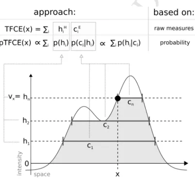
Figure 1. Illustration of the relation between the TFCE and the pTFCE approach. Both approaches are based on the integration of cluster-forming height threshold (h1, h2, …, hn) and the supporting section or cluster size (c1, c2, …, cn) at that given height. The difference is that, while TFCE combines raw measures of height and cluster size to an arbitrary unit, pTFCE realises the integration by constructing the conditional probability p(h|c) based on Bayes’ rule, thereby providing a natural adjustment for various signal topologies. Aggregating this probability across height thresholds provides enhanced P-values directly, without the need of permutation testing.
M AN US CR IP T
AC CE PT ED
P V ≥ ℎ2 | %2 = :;
<
;= 0 ℎ|%2 )ℎ
5
+ +>
, ?@ A ≥ ℎ2
1 , CℎDEF?GD
Eq. 3
142
, where v is the voxel value (Z-score) in the voxel of interest and the v<hi branch simply covers the 143
case of subthreshold voxels.
144
Here we propose, that a proper aggregation of the P(V≥hi|ci) probabilities over a hi series of 145
thresholds (0≤ hi <v, i=1, …, n), would satisfy our Enhancement property and Control property and 146
provide an appropriate way for integrating cluster information with voxel intensity. An illustration of 147
the “internal workings” of the proposed method can be seen in Figure 2 (parts A and B).
148
Probability aggregation across thresholds
149
The introduced conditional probability applies for the value of the actual cluster-forming threshold 150
instead of the value of the actual voxel. (As also suggested by the notation: P(V≥hi|ci) instead of 151
P(V≥v|ci)). That means that, when summarizing across thresholds, the aggregated probability should 152
be computed from an “incremental series” of probabilities (each of them corresponding a cluster- 153
forming threshold), rather than a pool of beliefs about the same event. Therefore, to aggregate the 154
P(V≥hi|ci) probability over all hi thresholds, the common probability pooling methods (Genest and 155
Zidek, 1986; Stone, 1961), e.g., logarithmic pooling, are not suitable.
156
To overcome this, in the following, we give a solution for this scenario, hitherto referred to as 157
equidistant incremental logarithmic probability aggregation. Our aim can be formalized as finding 158
an aggregation function Q(.), which exhibits the following properties:
159
(i) Q(.) is interpreted on the sum of a series of negative log-probabilities Pi, which are 160
equidistantly distributed in the logarithmic domain, and returns the negative logarithm 161
of the aggregated probability "H (With the sum of logarithms, we implement a 162
multiplicative model, see Appendix B and C of (Smith and Nichols, 2009)).
163
I: K − ! "2
2 → − ! "H ,
i = 1, 2, … , n; ∀?: ! "2 − log "2VW = % XGCYXC 164
Eq. 4
165
(ii) for the sum of a series of unenhanced –log P-values, P1=1 and Pn=P(V≥v)), Q(.) gives back 166
the negative logarithm of Pn, that is, the original voxel probability:
167
I Z K − ! "2
2 [ = I Z K − !# " \ ≥ ℎ2 (
2 [ = − ! "] ≅ − ! " \ ≥ A
Eq. 5
168
M AN US CR IP T
AC CE PT ED
169
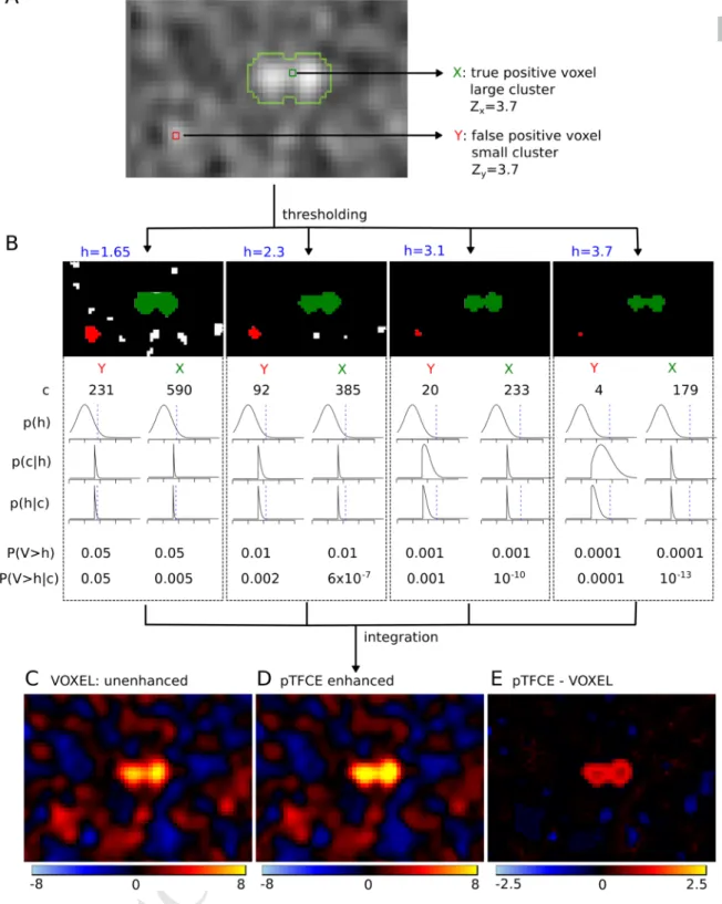
Figure 2. The “internal workings” of the pTFCE approach in a simulation case. Two voxels in a simulated image (signal 01 with SNR=1 and smoothing FWHM=1.5, see Evaluation Methods) with equal Z-score were chosen. One of them is part of a true signal artificially added to the smoothed noise image (denoted as X and with green colour), the other is random noise (Y, red). In part (A), the location of the selected voxels on the image is shown and the true positive areas are outlined with light green contour. Part (B) shows thresholded versions of the image (thresholds: h=1.65, 2.3, 3.1, 3.7, thresholds denoted by blue colour). The green and red clusters belong to voxels X and Y, respectively. For both clusters, the size of the cluster (c), the PDF of p(h) and the likelihood p(c|h) are plotted against Z-score thresholds on a range of [-2, 6]. Multiplying these and dividing by a normalizing constant gives the posterior p(h|c). Unenhanced (P(V>h)) and pTFCE-enhanced (P(V>h|c)) P-values are calculated for both voxels at each cluster forming threshold.
While enhanced P-values are only slightly different from the original unenhanced P-values for the random noise voxel Y, they exhibit a remarkable difference in the case of the true positive voxel X. In the pTFCE approach, these probabilities belonging to various thresholds are aggregated by an equidistant incremental logarithmic probability pooling approach (See section “Probability aggregation across thresholds” and Figure 3 for a geometric representation). Subtracting the unenhanced image (C) from the pTFCE enhanced image (D) reveals a remarkable intensity enhancement in the area of true signal.
M AN US CR IP T
AC CE PT ED
(iii) Q(.) is monotonically increasing, in the sense that it ensures monotonicity about local 170
maxima in the image.
171
Let us note, that our assumption about the constant increment in log probabilities in property (i) is 172
not obligatory for an appropriate aggregation method, but, as detailed below, by allowing a 173
mathematical analogy to the equation of triangular numbers, it simplifies the construction of a 174
proper aggregation method. Furthermore, the uniform sampling of the log(P) space is a natural way 175
to address a greater accuracy at small p-values, which are typically of interest.
176
In the followings, we introduce a Q function, which fulfils properties i-iii. Moreover, below we 177
present how the value Q(.) returns with the series of enhanced –log P-values as input (instead of the 178
original unenhanced ones, like in property ii) can be considered as the negative logarithm of the 179
pooled probability of interest:
180
I Z K − ! " \ ≥ ℎ2 |%2 &
2 [ ∶= 0
Eq. 6
181
As a starting point, let us consider the problem of finding the sum of the first n non-negative integer 182
numbers, which is `]= ∑]c db =] ]VW
e (giving the so-called triangular numbers). It is easy to 183
generalize this, instead of non-negative integers, to equidistantly distributed non-negative real 184
numbers from 0 to nΔk and by an increment of Δk: 185
`∆g, ]∆g = K b∆c=X∆c X + 1 2
]
c d = X∆ciX∆∆cc+ 1j
2
Eq. 7
186
If we use the notation w=nΔk and denote `∆g,]∆g as simply S, we can write Eq. 7 as:
187
0 = 1
2∆cFe+1 2 F + `
Eq. 8
188 189
Solving Eq. 8 for w and taking the positive root gives:
190
FV= l∆c 8S + ∆c − ∆c
2 ∶= I S
Eq. 9
191
In the context of our pTFCE approach, let S(x) denote the sum of the –log P(V≥hi |c) enhanced log- 192
probabilities in voxel position x, so that the hi thresholds change incrementally in the negative 193
logarithmic domain (to ensure a constant Δk):
194
M AN US CR IP T
AC CE PT ED
S x = K − log#P V ≥ ℎ2 |%2 ( ?X A D 0 G?C? X
qr
2 d
196
and 197
∀i, 0 ≥ i > *+ ∶ log " \ ≥ ℎ2VW − log " \ ≥ ℎ2 = ∆c
Eq. 10
198
The proposed I ` probability pooling for pTFCE clearly satisfies (i), (ii), (iii) of the above 199
conditions. Let us note, that the formulation of the introduced probability aggregation method forces 200
the starting -logP threshold to be zero (P1=1) and, importantly, the number of thresholds and the 201
maximal threshold does only affect the accuracy of the approximation as we normalise for ∆c and 202
the enhanced –log P-values are zero for subthreshold voxel.
203
The rationale of the proposed equidistant incremental logarithmic probability aggregation method 204
can be understood as searching for the probability corresponding to a hypothetical A′ voxel value for 205
which the threshold-wise unenhanced sum of negative log probabilities would be the same as the 206
actual enhanced sum corresponding to the observed voxel value v.
207
Another, analogous and even more straightforward way to think about the method is that it links the 208
series of enhanced probabilities produced by a “strongly clustered” voxel to another hypothetical 209
series of probabilities produced by a higher intensity voxel, but with “average” clustering (relative to 210
smoothness) where, accordingly, enhancement has no effect at all; and uses this higher intensity as 211
the pooled (and enhanced) intensity value.
212
It can be also intuitive to consider a geometric meaning of the method as demonstrated on Figure 3. 213
Computing the pooled log probability pTFCE(x) of voxel x by the Q function is equal to finding the 214
hypothetical voxel value, for which the sum of the unenhanced (original) incremental log probability 215
series ( SΔk, v’ according to Eq. 7, denoted as S’orig and the blue area on the figure) is equal to the sum 216
of the pTFCE enhanced log probability series belonging to the actual (observed) voxel intensity v 217
(denoted as S’orig and the red area on the figure).
218
M AN US CR IP T
AC CE PT ED
Let us note that, up to this point, our formulation of the pTFCE approach does not contain any detail 219
about the data structure and it can be easily generalized to various features of the data beside 220
clustering. In the next section, we link the introduced formulation to the typical volumetric data 221
structure in neuroimaging by estimating the appropriate PDFs based on Gaussian Random Field 222
Theory.
223
Estimating the likelihood function
224
We see at least two obvious ways for determining or approximating the probability density functions 225
p(h) and p(c|h) in order to construct the P(V≥h), P(C≥c|h) and P(V≥h|c) probabilities: for n- 226
dimensional images, the PDFs in question can be approximated based on Gaussian Random Field 227
(GRF) theory, and in general, empirical estimation of the PDFs can be given by statistical resampling 228
or permutation test. Since GRF theory (Bardeen et al., 1986; Nosko, 1969) is extensively used in 229
statistical analysis of medical images (Friston et al., 1996; Nichols, 2012; Worsley et al., 2004), in the 230
present work, we choose to investigate the use of GRF Theory to give an approximation of the PDFs 231
and use simulations with a known ground truth to justify the validity of the approximation. Let us 232
note however, that the use of GRF theory makes our approach specific to 3D images and implicitly 233
introduces several assumptions not involved in the above discussed general formulation. While the 234
GRF-based approach is well suited to establish the links of pTFCE to the existing practice in the field 235
of neuroimaging, more general formulations (like the use of permutation-based empirical 236
distributions) are subject of further investigation in order to fully exploit the generalisable 237
formulation of the core pTFCE approach.
238
Determining p(h) for a given threshold h (or p(v) if v is the voxel value) for Gaussianised Z-score 239
images is straightforward: it is simply the PDF of the normal distribution with zero mean and unit 240
variance:
241
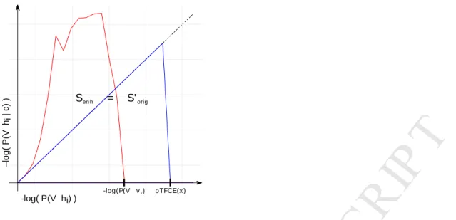
Figure 3. Geometric representation of the proposed equidistant incremental logarithmic probability pooling approach.
The proposed equidistant incremental logarithmic probability aggregation method links the series of enhanced probabilities produced by a “strongly clustered” voxel (red area, Senh) to another series of probabilities produced by a hypothetical, higher intensity voxel, but with “average” clustering (blue area, S’orig), where enhancement has no effect at all; and uses this higher intensity as the pooled (and enhanced) intensity value.
.
-log( P(V hi) )
–log( P(Vhi | c) ) Sen h = S'orig
pTFCE(x ) -log(P(V vx)
M AN US CR IP T
AC CE PT ED
Eq. 11
243
, where u (uppercase) is the cumulative distribution function and t (lowercase) is the probability 244
density function of the standard Gaussian. Note that, according to Eq. 11, we define the input image 245
for pTFCE as an image of Z-scores, nevertheless, it is easy to convert any other statistical parametric 246
images (like T- or P-values) to Z-scores.
247
For inference on clusters, we first utilize GRF theory to find the mean cluster size under the null at a 248
given threshold, the distribution of cluster size about that mean and also, the P-value for a given 249
cluster size.
250
Let N be the total supra-threshold volume (equivalently, the sum of all of the cluster sizes); let L be 251
number of clusters observed. Assuming a large search region relative to the smoothness, and thus 252
independence of number of clusters and cluster size, the mean cluster size under the null is 253
v w = v*w/ vyw. Here, the numerator is easily obtained: EvNw = \ P V ≥ h , and specifically for 254
a Gaussian image: EvNw = \ 1 − u ℎ , where u . is the CDF of a Gaussian and V is the total 255
number of voxels (Friston et al., 1996).
256
The expected number of clusters is E[L] approximated by the expected Euler Characteristic (Worsley 257
et al., 1996). The Euler Characteristic (EC) of a D-dimensional random field thresholded at h is written 258
χh, and is the number of clusters minus the number of holes (D≥2) plus the number of handles (D≥3).
259
For sufficiently high h the probability of a hole or handle is small, and so the EC offers a good 260
approximation of the number of clusters. Worsley's general results (Worsley et al., 1996) give a 261
closed-form expression for E[χh] as a sum of D terms: v~+w = ∑•€ d•€‚€ ℎ , where Rd is the RESEL 262
count and ρd is the EC density. The RESEL count is a length, area or volume, depending on d, and it is 263
the product of the spatial measure and a roughness measure |Λ|1/2, where Λ is the d × d variance- 264
covariance matrix of the partial derivatives of the data. Usually, only the d = D term is appreciable, so 265
for the 3D case we have v~+w = •ƒ ℎe− 1 D6+„…e 2† 6‡ e… . Thus, the expected cluster size for a 266
3D Gaussian (Z-score) image with cluster-forming threshold h is:
267
v%+w = \ 1 − u ℎ
\ |ˆ|We ℎe− 1 D6+e„ 2† 6e= \ 1 − u ℎ
•• ℎe− 1 D6+e„ 2† 6e
Eq. 12
268
Finally, using the result that cluster size to the 2/D power follows an exponential distribution (Nosko, 269
1969), with 270
‰+ = Š v%w Г iŒ2 + 1j •
6e•
Eq. 13
271
, the PDF of the cluster size at threshold h is:
272
0 %|ℎ =2‰+D6Žr „ •… 3%W ƒ…
, and 273
M AN US CR IP T
AC CE PT ED
" > %|ℎ = %e ƒ…D6Ž „ •…
Eq. 14
274
, where λ is the rate of the exponential distribution and Γ(·) is the gamma function.
275
There are several implicit assumptions in the Gaussian Random Filed approach (Friston et al., 1996), 276
and, importantly, GRF theory-based estimates become inaccurate or even undefined at low 277
thresholds. Therefore, for the GRF-based implementation of pTFCE, here we propose that for any 278
thresholds h smaller than a specific value hGRF, the enhanced probability P(H>h |c) is to be 279
approximated simply by the unenhanced P(H>h). Moreover, in Eq. 2, 0 %|ℎ should be truncated by 280
setting it to 0 when h< hGRF. Let us note, that this also truncates the resulting 0 ℎ|% distribution on 281
the left side, thus slightly increases the enhanced probability " \ ≥ ℎ |% , meaning that with this 282
approximation, the cluster enhancement is expected to be conservative. That also means that, while 283
this approximation might mean a loss in sensitivity, we can still expect our pTFCE approach to 284
perform well in terms of our Control property (that is, it remains controllable e.g., for family wise 285
error). Investigation of the effect of hGRF for using GRF theory revealed that the pTFCE is robust to the 286
choice of this value (see Supplementary Figure 5). Therefore, we fixed this value at hGRF=1.3 (default 287
parameter in the software implementations, as well), and tested the validity of this approximation in 288
simulations with known ground truth and on real data.
289
Evaluation Methods
290
1.3 Simulated data
291
To assess the statistical validity of our methods, simulated data comprising seven 3D test image 292
shapes (the same as in (Smith and Nichols, 2009)) were used to compare the pure voxel-level (a.k.a.
293
unenhanced, hereinafter denoted simply as “VOXEL” method), the TFCE and the proposed pTFCE 294
methods against each other, with ROC evaluations giving objective combined measures of specificity 295
and sensitivity. Additionally, we tested whether the P-values output by the pTFCE method are valid 296
for correction for multiple comparisons, by correcting based on the P-value distribution of the 297
unenhanced voxel-based approach (See ROC methodology). This method we denote as pTFCEVOX, to 298
emphasize that is uses the thresholds computed for the VOXEL method and to distinguish it from the 299
variant with the randomisation-based threshold (denoted simply as pTFCE).
300
1.3.1 Test signal shapes
301
In our simulations, we used the same seven 3D test signal shapes as in (Smith and Nichols, 2009).
302
These are shown on Error! Reference source not found.A. These ground truth images cover a wide 303
range of signal types, including small blobs, touching blobs and extended areas of activation. Each 304
test signal has a background value of 0 and a peak height of 1. We then scaled the signal by a factor 305
or 0.5, 1, 2 or 3 and added unsmoothed Gaussian white noise of standard deviation 1, to give a range 306
of peak signal-to-noise (SNR) values: 0.5, 1, 2 and 3.
307
We evaluated also the effect of different Gaussian smoothing kernels, with full-width-at-half- 308
maximum (FWHM) values of 1, 1.5, 2, 3 voxels applied. After smoothing, the data was scaled so as to 309
M AN US CR IP T
AC CE PT ED
An ROC (receiver-operator characteristic) curve, given a signal+noise image and the known ground 313
truth, plots true positive rate (TPR) against false positive rate (FPR), as one varies a threshold applied 314
to binarise the image. An ideal algorithm gives perfect true positive rate at zero false positive rate, 315
i.e., the perfect ROC curve jumps immediately up to TPR=1 (y-axis) for FPR=0 (x-axis) and stays at 1 316
for all values of FPR. Hence a commonly-used single summary measure of the whole ROC curve is the 317
AUC (area under curve); the higher the AUC, the better. To ease interpreting our results in relation to 318
those in (Smith and Nichols, 2009), we use an analogous ROC methodology: we use AUC values for 319
alternative free-response receiver-operator characteristic (AFROC) (Bunch et al., 1977; Chakraborty 320
and Winter, 1990).
321
Alternative free-response ROC 322
AFROC analysis plots the proportion of true positive tests (among all possible positive tests) on the y- 323
axis and the probability of any false positive detections anywhere in the image on the x-axis (that is, 324
the family-wise error rate, or FWER). Here we calculate FWER for the AFROC curves by counting the 325
number of images with one or more false positive voxels among 1000 smoothed noise-only images.
326
As neuroimaging analyses typically seek to control the FWER, we used this method to test the 327
Enhancement property of different spatial enhancement/thresholding methods. For AFROC analysis, 328
we define true positives based on the smoothed ground truth images.
329
Since ROC analysis is predominantly a binary concept, we threshold and binarise the smoothed 330
ground truth images at 0.1/SNR. This ensures, that voxels, in which a significant amount of signal was 331
introduced by smoothing, count as true positive observation, if detected by any of the methods.
332
The above approach of calculating AFROC, by estimating FWER from processed pure-noise data, 333
avoids the need to determine what is “real” background in the signal+noise data after passing 334
through a given algorithm (Smith and Nichols, 2009). It is exactly what we want in the standard 335
scenario of null-hypothesis testing which aims to explicitly control the FPR in the presence of no true 336
signal; it tests sensitivity when the specificity is being controlled globally (that is among studies and 337
not over voxels), in the way that we generally require in practice. This method of calculating FWER 338
ignores the FP voxels in the signal+noise images that are spatially close to the true signal (as distinct 339
from “real” FP voxels in the noise-only data), and in doing so does not weight, for example, against 340
the smearing of estimated signal into neighbouring voxels due to smoothing.
341
“Negative” alternative free-response ROC 342
Since FWER for AFROC is calculated from the noise-only images, aside from the effect of smoothing, 343
AFROC is insensitive to “cluster leaking”, as well. This might be an undesirable property since 344
“leaking” will possibly merge small blobs of activity with neighbouring random local maxima and 345
present them as large clusters with lots of false positive voxels (Woo et al., 2014). Therefore, while 346
AFROC is suitable for measuring signal detectability, to control for the voxel-level spatial specificity of 347
the methods, here we introduce the “negative AFROC” method.
348
In the negative AFROC (short: nAFROC) analysis, we test our Control property for “cluster leaking”, by 349
thresholding the smoothed ground truth images also at 0.001/SNR and then binarising and inverting 350
it to define a region where the amount of signal can be neglected. Applying our AFROC method with 351
this region as ground truth, we create ROC curves for the FPR, plotted against the FWER. An 352
appropriate cluster enhancement algorithm should keep the area under the negative AFROC curve 353
very close to zero, to minimise voxel-level Type I errors.
354
Correcting for multiple comparisons on enhanced probability values 355
As the introduced pTFCE enhancement method directly outputs probability values, we also tested 356
whether these enhanced probability values can indeed be interpreted in the range of the original, 357
M AN US CR IP T
AC CE PT ED
unenhanced probability values (Control property: multiplicity) that is, thresholds corrected for 358
multiple comparisons on the original, unenhanced data are directly applicable to the pTFCE 359
enhanced data, as well. We did this by using the unenhanced noise-only images to calculate the 360
FWER thresholds for the AFROC and negative AFROC curves. The rationale behind this analysis is that 361
if thresholds computed from, and interpretable on unenhanced data are valid on pTFCE-enhanced 362
probability values, as well (that is, they always guarantee a smaller or equal FWER), then a freedom 363
in the choice of the correction method is granted, as long as it is valid on the original statistical 364
image. In practice this would mean that no special correction methods for enhanced images (like 365
permutation test-based maximum height correction) are needed and any threshold will give an equal 366
(or close) FWER for the enhanced image than for the unenhanced.
367
We denote this analysis case, as pTFCEvox, the subscript standing for VOXEL and referring to the way 368
corrections for multiple comparisons were based on the P-values of the (unenhanced) voxel-level.
369
1.3.3 Simulation details
370
To summarize, our simulation and ROC analysis consisted of the following steps:
371
1. Generate the raw ground truth 3D image (“signal”).
372
2. Generate 1000 random Gaussian noise images (mean zero, unit variance) that, when added to the 373
signal, give a specified SNR in the resulting 1000 signal+noise images. We applied exactly the same 374
noise realizations as in (Smith and Nichols, 2009) and generated signal+noise images for SNRs 0.5, 1, 375
2 and 3.
376
3. Pass all noise-only and signal+noise images through a smoothing stage (with FWHMs 1, 1.5, 2 and 377
3) and afterwards, through the algorithm being tested: VOXEL (=no enhancement), TFCE, pTFCE, 378
pTFCEvox (=pTFCE at this stage).
379
4. Pass also the ground-truth image through the smoothing stage, normalise its intensity to max=1, 380
and threshold it at 0.1/SNR and binarise, to define a ROI of true positive observations. The rationale 381
behind smoothing the ground truth image is, that “de-smoothing” should not be the responsibility of 382
any statistical inference method. Similarly, when smoothing is applied in a real data scenario, we can 383
only expect to detect the smoothed version of the underlying activation pattern (which is also a 384
strong argument against using excessive smoothing). Accordingly, areas of false positive observations 385
are also defined based on the smoothed ground truth image, by thresholding it at 0.001/SNR, and 386
then binarising and inverting it.
387
5. Compute the traditional ROC curves for the processed signal+noise images and for the ground 388
truth mask thresholded at 0.1/SNR.
389
6. Compute AFROC and negative AFROC curves: threshold the appropriately processed noise-only 390
and signal+noise images for the methods voxel, TFCE and pTFCE and pTFCEvox at the full range of 391
possible threshold values. FWER, TPR and FPR at each threshold are computed as follows:
392
• FWER: For each threshold level, count the number of processed noise-only images which contain 393
any supra-threshold voxels. This count (divided by 1000) gives the family-wise FPR for this threshold 394
level (i.e., achieves full correction for multiple comparisons across space). For pTFCEvox, FWER is 395
M AN US CR IP T
AC CE PT ED
signal+noise images (we also record the IQR of the TPR across the 1000 images, as a measure of the 400
stability of the various algorithms being tested).
401
• FPR: For each threshold level, use each of the 1000 processed signal+noise images, and use the 402
“negative” ground truth mask (thresholded at 0.01/SNR, binarised and inverted) to obtain an 403
estimate of the FPR. The raw voxel-wise FPR is then averaged across the 1000 images (again, we 404
record the IQR, as well).
405
6. Take the resulting ROC, AFROC and negative AFROC curves, and, using only the x-range of 0 to 406
0.05, calculate the AUC values (AUC ROC, AUC AFROC, AUC negative AFROC, respectively). Normalise 407
AUC by 0.05.
408
For an example of ground truth smoothing and the ROIs used for the ROC methodology along with 409
demonstrative results of the tested approaches, see Figure 4.
410
For estimating smoothness of the signal+noise images, for generating signal+noise images and for 411
AFROC analysis, we used FSL (Jenkinson et al., 2012; Smith et al., 2004). (We performed a 412
“traditional” ROC analysis, as well, see Supplementary Figure 2 and Supplementary Table 1) The 413
pTFCE algorithm was implemented in R, using the packages “mmad” (Clayden, 2014) (used for a fast 414
labelling of connected components in thresholded images) and “oro.nifti” (Whitcher et al., 2011) (to 415
manipulate nifty images). Calculation of pTFCE was performed with a fixed number of log(P)- 416
thresholds (n=100), ranging from 0 to the negative logarithm global image maximum − ! max& A& , 417
and distributed equidistantly. Although this results in different deltas for various images, theory 418
suggests that this affects only the accuracy of the probability aggregation and our supplementary 419
analysis (Supplementary Figure 3) confirmed that the proposed equidistant incremental logarithmic 420
probability aggregation method is robust above a reasonable number (n≥100) of thresholds and 421
magnitude of delta values. Overflow problems were handled in most of the cases in the same way as 422
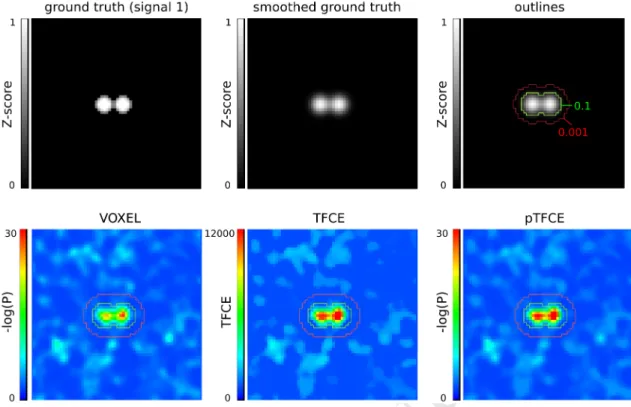
Figure 4. Representative images of the simulation and ROC ROIs for the investigated approaches. In the upper row, the unsmoothed and the smoothed (FWHM=1.5) versions of signal 2, and the outlines corresponding to the ROC (inside vs. outside the 0.1 contour), AFROC (inside the 0.1 contour) and negative AFROC (outside the 0.001 contour) analysis. In the lower row, results of the VOXEL, TFCE and pTFCE methods with the same noise realisation (noise 0001) are visualized with the contours as overlay.
M AN US CR IP T
AC CE PT ED
in the FSL source code (Jenkinson et al., 2012; Smith et al., 2004). Results were plotted with the 423
oro.nifti and the ggplot2 (Wickham, 2016) packages of R. We compare the AUC values at identical 424
parameter settings. Moreover, since it is a common practice to optimise neuroimaging pipelines in 425
terms of smoothing to achieve maximal sensitivity, and optimization often implicitly takes into 426
account the typical signal-to-noise level of the experimental design (through the inherent properties 427
of the data used to optimise the workflow), for each method, each test signal and each SNR, we 428
chose an optimal smoothing based on the best AUC values of the AFROC curves and compared 429
methods with their optimal settings.
430
1.4 Testing on real data
431
Since real neuroimaging data differs in many properties from the simplistic Gaussian model used in 432
the simulation, we use various fMRI datasets for the purposes of (1) evaluating the improvement in 433
sensitivity by investigating the dependence of results on sample size, (2) investigating whether pTFCE 434
maintains nominal family-wise error rates when corrected for multiple comparison, given that the 435
null hypothesis is true; and (3) illustrate the effect of pTFCE with enhancing the activation map 436
reflecting the pain matrix which is well known and complex enough to capture the advantages of our 437
method. We took advantage of the easy correction of pTFCE P-values for multiple comparisons and 438
did not apply the permutation-based FWER thresholds for pTFCE; only the pTFCEvox method 439
(maximum-height thresholding based on GRF-theory) was tested in the real-data scenarios.
440
1.4.1 Demonstration of the increased statistical power on real data
441
For both the demonstration of increased statistical power and the evaluation of family-wise error 442
rates, we obtained data from the UCLA Consortium for Neuropsychiatric Phenomics LA5c Study (CNP) 443
(Gorgolewski et al., 2017; Poldrack et al., 2016) as shared via the OpenNeuro database (accession 444
number: ds000030, https://openfmri.org/dataset/ds000030/). Processed 1st-level activation maps 445
(contrast of parameter estimates, a.k.a “cope” images, as provided with the dataset) of N=119 446
healthy participants from the “switch-noswitch” contrast (cope39) of the task switching paradigm 447
were obtained and fed into FSL “randomise” (number of permutations: 5000) to create a group- 448
mean activation map. This activation map was then thresholded at a voxel-level (unenhanced) FWER- 449
corrected p<0.05 threshold and considered as “ground truth” for further analysis. As a next step, a 450
total of 900 activation maps were computed from random subgroups of the healthy population with 451
sample sizes N=5, 10, 20, 30, 40, 50, 60, 80 and 100 and with 100 random sampling per sample size.
452
Corrected (FWER, p<0.05) voxel-level and TFCE images and T-score maps were obtained. The latter 453
ones were converted to Z-score maps, fed into the pTFCE algorithm and thresholded based on GRF 454
theory, with a corrected threshold of p<0.05 (implementing the pTFCEvox approach). True positive 455
rate was defined as the proportion of “ground truth” voxels found by the thresholded activation 456
maps of the subsamples. Mean, 0.025% and 0.975% percentiles of this true positive rate were 457
obtained for each of the investigated methods (VOXEL, TFCE and pTFCEvox) and plotted against the 458
sample sizes.
459
1.4.2 Evaluation of family-wise error rates on real data
460
Evaluation of family-wise error rates in the case of a true null hypothesis was performed on the same 461
dataset as the demonstration of statistical power (CNP study, OpenNeuro database, ds000030). The 462
true null hypothesis (no group difference) was approximated by comparing 1st-level activation maps 463
(contrast of parameter estimates, a.k.a “cope” images, as provided with the dataset) of two random 464
M AN US CR IP T
AC CE PT ED
and thresholded based on GRF theory, with a corrected threshold of p>0.05 (implementing the 470
pTFCEvox approach). Family-wise error rate for each method was than estimated by the ratio of 471
thresholded images with any non-zero value across the 1000 random comparisons, for each method.
472 473
1.4.3 Illustration of the cluster enhancement effect
474
For the illustration of the cluster enhancement effect, we used data published as part of (Bingel et 475
al., 2011). This study investigated how divergent expectancies alter the analgesic efficacy of a potent 476
opioid in healthy volunteers by using fMRI. We aimed to evaluate enhancement approaches on the 477
published group-mean map of brain activation to painful stimulation, activating the pain matrix 478
(Figure 3. of the paper).
479
For TFCE, we fed the appropriate spatially standardized subject-level SPM contrast images into 480
randomise and estimated TFCE-enhanced, FWER-corrected p-values for the group mean activation 481
(number of permutations: N=10000). For pTFCE, we simply obtained the corresponding second-level 482
spmT image (see (Bingel et al., 2011) for details) and converted it to Z-score, based on the degrees of 483
freedom (dof=63). We estimated the smoothness of the map with the “smoothest” command-line 484
tool of FSL. The Z-score map and the smoothness estimate was then fed into the pTFCE algorithm 485
which computed the enhanced map (outputting negative log P-values). The working resolution of the 486
data in standard space was 2×2×2 mm for both TFCE and pTFCE. For visualization, the original and 487
the enhanced negative log P-value maps were thresholded at 13.61, the –log(P) threshold 488
determined by the FWER correction (P<0.05) in the original study. The FWER correction for TFCE was 489
based on the permutation test.
490
M AN US CR IP T
AC CE PT ED
Results
491
1.5 Implementation details
492
The pTFCE algorithm is available as an R package called “pTFCE”, and also as an SPM (Friston et al., 493
1994a) Toolbox with the same name. These packages, together with a fast C++ and FSL-based 494
implementation and nipype interfaces (Gorgolewski et al., 2011) are also available at 495
https://spisakt.github.io/pTFCE.
496
1.6 Simulation results
497
The full AFROC curves (See Error! Reference source not found.C for some representative curves) 498
reveal that our AUC results are not dependent on the applied x-axis threshold (FWER P<0.05), since 499
all curves have a smooth rise in the 0-0.05 interval and differences between approaches are constant 500
at nearly all FWER thresholds. Therefore, AUC values provide valid description of these curves in the 501
following sections.
502
1.6.1 Comparing enhancement methods with optimal parameter settings
503
It is common practice to optimise neuroimaging pipelines in terms of smoothing to achieve maximal 504
sensitivity. Moreover, optimization often implicitly considers the typical signal-to-noise level of the 505
experimental design. Therefore, besides comparing all tested methods with identical parameter 506
settings (section 1.6.2), for each method, each test signal and each SNR, we chose an optimal 507
smoothing, based on the best AUC values of the AFROC curves. Results for SNR=1 and 2 are plotted 508
in Figure 6.
509
The mean(±sd) optimal smoothing FWHM across all test signal shapes and SNR values was 510
2.29(±0.65), 1.86(±0.84), 2.02(±0.78) and 1.96(±0.76) voxels for VOXEL, TFCE, pTFCE and pTFCEvox, 511
respectively. Although pooling across test signal shapes obviously does not necessary provide 512
summary statistics that are representative for real experimental settings, these results still strongly 513
suggest that the cluster enhancement methods generally require less smoothing. Not surprisingly, in 514
the case of spatially extended test signal shapes (signals 3, 6 and 7) a greater smoothing was 515
preferred by all methods. In the case of the other, spatially more restricted signal shapes (signals 1, 516
2, 4 and 5) an optimal smoothing of 1 or 1.5 was found. TFCE preferred in several instances an even 517
smaller smoothing than pTFCE and pTFCEvox. 518
In general, when pooled over all ground truth images and all SNRs, pooled mean(±sd) for the mean 519
AUC of AFROC curves with optimal smoothing were 0.102(±0.16), 0.141(±0.2), 0.142(±0.2) and 520
0.134(±0.2) for VOXEL, TFCE, pTFCE and pTFCEvox, respectively, clearly underpinning the 521
improvement in sensitivity in the case of cluster enhancement methods. Moreover, with optimal 522
smoothing, pTFCE and pTFCEvox outperformed the unenhanced inference for all SNR values and 523
ground truth shapes. TFCE did not manage to improve sensitivity in case of test signals 1, 2 and 5 524
with large SNR values. Summarising the inter-quartile ranges suggests that pTFCE and pTFCEvox (mean 525
IQRs 0.018, 0.02) might be somewhat more robust than TFCE (0.022), but the unenhanced inference 526
displayed the strongest stability (0.013).
527
M AN US CR IP T
AC CE PT ED
When comparing the FWER-controlled sensitivity of cluster enhancement methods against each 528
other, we found that pTFCE and pTFCEvox outperforms TFCE in almost all cases with spatially more 529
restricted test signals (signal 1, 2, 4 and 5). This difference is present already at SNR=1, but becomes 530
more expressed with greater SNR. In contrast to pTFCE and pTFCEvox, TFCE preferred ground truth 531
images with spatially extended signal. With these ground truth images, it produced remarkably 532
greater AUC values in AFROC analysis than pTFCE. However, we observed an increased number of 533
probably “cluster leaking”-related false positives in these cases. Notably, a modest increase of false 534
positives was experienced also in case of pTFCE and pTFCEvox, but AUC values of nAFROC curves were 535
significantly lower than for TFCE (second row in each panel of Figure 6). For the aforementioned 536
spatially restricted test signals, all cluster enhancement methods give very strict control over cluster- 537
leaking and corresponding false positives, as shown by the nAFROC curves and corresponding AUC 538
values.
539
The AUC values of pTFCEvox are systematically slightly below the mean AUC values of pTFCE, but, 540
relative to the other methods, are not very much lower. This suggests that correcting GRF-based 541
enhanced pTFCE P-values for multiple comparisons gives valid results even if it is based on the 542
distribution of the unenhanced P-values (“VOXEL” noise images instead of “pTFCE noise images”).
543
1.6.2 Comparing enhancement methods with identical parameter settings
544
Another possible concept for contrasting the tested approaches is to investigate their performance 545
with identical parameter settings, instead of using the optimized smoothing values for each. Separate 546
comparison of the tested approaches with each parameter-setting showed, in general, very similar 547
results to those revealed with optimized smoothing.
548
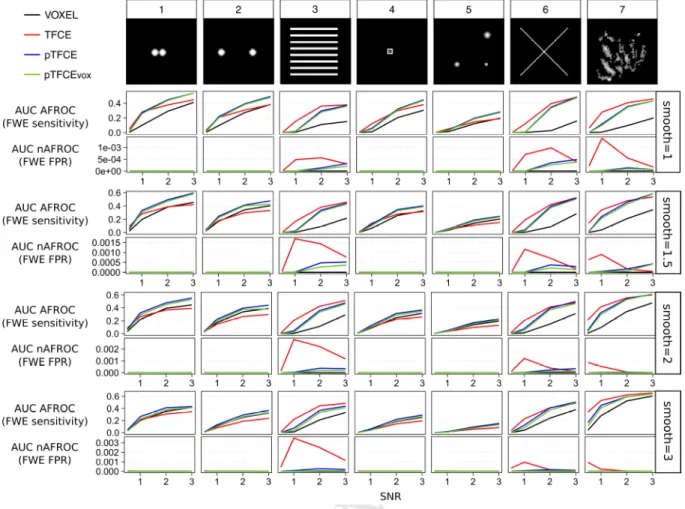
Figure 5. AUC values of the AFROC (representing FWER-level sensitivity) and negative AFROC (representing 1-FWER-level specificity) curves for all methods, ground truth shapes, SNRs, with the optimal smoothing. Barplots represent the mean across 1000 simulation runs, and whiskers represent the inter-quartile range.
M AN US CR IP T
AC CE PT ED
In these comparisons, as well, cluster enhancement methods tended to be superior to the 549
unenhanced voxel-level inference (Figure 7, AUC AFROC: upper row for each smoothing value), 550
although again, in a few cases (typically for high SNRs with test signals 1, 2 and 5) TFCE yielded lower 551
mean AUC values than unenhanced voxel-level thresholding with the same simulation parameters.
552
On the other hand, pTFCE robustly outperformed the unenhanced thresholding in all of the 553
simulation parameter settings. The same is true for pTFCEvox suggesting that thresholding the pTFCE 554
enhanced image with thresholds originally interpreted on the unenhanced image also results in an 555
enhanced sensitivity.
556
The mean area under the negative AFROC curve is, for most of the parameter settings, relatively 557
close to zero, meaning an appropriate control for false positives and “cluster leaking”. However, in 558
case of the cluster enhancement methods (TFCE, pTFCE and pTFCEvox), false positives (defined by our 559
nAFROC analysis, very conservatively, as regions where the noise is at least 1000 times greater than 560
signal) slightly accumulate by ground truth images with extended area of signal (signals 3, 6 and 9, 561
upper row of each smoothing parameter panel on Figure 7).
562
When comparing cluster enhancement methods against each other, we found a very similar pattern 563
to that with optimized smoothing: pTFCE and pTFCEvox tended to slightly outperform TFCE in terms of 564
FWER-controlled sensitivity in almost all cases with spatially more restricted test signals (signals 1, 2, 565
Figure 6. Mean AUC values of the AFROC (representing FWER-level sensitivity) and negative AFROC (representing 1-FWER- level specificity) curves for all methods, ground truth shapes, SNRs and smoothing kernels.