O R I G I N A L S T U D Y
An improved torque type gravity gradiometer with dynamic modulation
Jie Luo1•Jia-Hao Xu1•Qi Liu2•Cheng-Gang Shao3• Lin Zhu3•Hui-Hui Zhao3•Wei-Huang Wu1
Received: 29 December 2016 / Accepted: 7 July 2017 / Published online: 24 July 2017 Akade´miai Kiado´ 2017
Abstract Traditional torque type gravity gradiometer has an important pole in gravity gradient measurements, while it is relatively inefficient and with the precision of about 1 E mainly caused by the static operating mode. In this paper, we develop an improved torque type gravity gradiometer to improve the measuring efficiency, which is based on the dynamic modulation. The dynamic modulation keeps the gradiometer rotating on a turntable steadily, measures the deflection angle of the torsion pendulum continuously and then obtains the gravity gradients. The result shows that after using the improved gra- diometer, the gradients WxzandWyz are obtained with precisions of 0.45 E and 0.32 E respectively in a cycle of 20 min.
Keywords Improved torque type gradiometerDynamic modulationMeasuring efficiencyGravity gradient
1 Introduction
The gravity gradient measurement can offer an efficient way for resource explorations in earth (Zhou et al.2015; Vo¨lgyesi2001). The torque type gradiometer was widely applied to the oil field exploration in the past (Bell and Hansen1998; Szabo´2016), because the
& Qi Liu
louis_liuqi@mail.hust.edu.cn
& Cheng-Gang Shao
cgshao@mail.hust.edu.cn
1 School of Mechanical Engineering and Electronic Information, China University of Geosciences, Wuhan 430074, China
2 TIANQIN Research Center for Gravitational Physics, School of Physics and Astronomy, Sun Yat- sen University, Zhuhai 519000, China
3 MOE Key Laboratory of Fundamental Physical Quantities Measurement, School of Physics, Huazhong University of Science and Technology, Wuhan 430074, China
https://doi.org/10.1007/s40328-017-0202-z
gravity gradient data could be used to reveal underground mass distribution. The torque type gradiometer designed by Eo¨tvo¨s made a great difference on the petroleum industry in early twentieth century (Barton1931; DiFrancesco et al.2009; Shaw and Lancaster-Jones 1922). The equilibrium position and torsional motion of the pendulum in this type gra- diometer were found to be remarkably stable and relatively constant, so that the instrument could be used not only in a well-protected laboratory, but also in a field (Shaw and Lancaster-Jones1922). However, the gravity gradient measurement with the Eo¨tvo¨s torque type gradiometer needs a long time to record the deflection angle of the torsion pendulum.
The observation using this type gradiometer should be done in the night of stable mea- surement environment (Szabo´2016), since it is easily affected by the external environment variations, such as temperature fluctuation, barometric pressure change and so on. There have been many successive improvements on the instrument structure and measuring process, while all these relative observations with the static operating mode need a long measurement cycle (Schweydar1918; Rankine1932). The gravity gradients given by the torque type gradiometer should be determined by observing at least five different azimuth angles (Bell and Hansen 1998), the observers must alternate the azimuth angles of the gradiometer by a turntable with manual and later automatic operations (Vo¨lgyesi2015), and besides the formal observation starts after the torsion pendulum reach to the stable state. Typically, the torsion pendulum has a period of swing exceeding twenty minutes (Rankine1932). These above factors result in the relatively low efficiency of this type gradiometer. Then, for this traditional torque type gradiometer, the gravity gradients could be obtained with a precision of 1 E after 12 h observation (Shaw and Lancaster- Jones1922).
In order to improve the measurement efficiency and accuracy, we develop an improved torque type gradiometer with dynamic modulation mode to determine the gravity gradients.
The torsion pendulum is placed on a stable turntable, which rotates continuously at a constant velocity during the observation, and then we can obtain a set of gravity gradients from every rotating cycle. In addition, the torsion pendulum is free to twist, and the useful signal is modulated on the measurable deflection angle (Luo et al. 2013). Therefore, compared to the traditional Eo¨tvo¨s torque type gradiometer with the static operating mode, the torsion pendulum of the improved gradiometer can observe the deflection angle of the pendulum continuously and measure gravity gradients in a short period of the turntable.
Due to the short measurement cycle, this improved Eo¨tvo¨s torque type gradiometer can avoid unnecessary noises and disturbances. In this paper, we propose the principle of the improved gradiometer, describe the design of the relative instrument, and analyze the influences of the thermal noise and irregularity in the rotation rate on the estimation of the gravity gradients. Finally, we process a typical data set of the measurement of the gravity gradients with the improved torque type gradiometer, then obtain the values and uncer- tainties of the gravity gradients, and further make contribution to the determination of the gravity gradients.
2 Principle of the improved torque type gradiometer with dynamic modulation
2.1 Gravity gradient
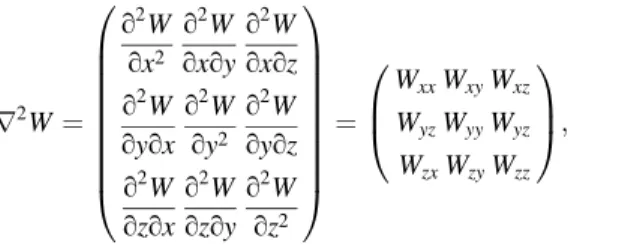
W¼VþU; ð1Þ whereVis the gravitational potential,Uis the potential of centrifugal force. There are 9 s order partial derivatives ofWin a cartesian coordinate system, expressed as:
r2W¼ o2W
ox2 o2W oxoy
o2W oxoz o2W
oyox o2W
oy2 o2W oyoz o2W
ozox o2W ozoy
o2W oz2 0
BB BB BB BB
@
1 CC CC CC CC A
¼
WxxWxyWxz
WyzWyyWyz
WzxWzyWzz
0 B@
1
CA; ð2Þ
where the five componentsWxx,Wxy,Wxz,Wyy, andWyzare independent, since the earth gravity field is an irrotational field and the three diagonal components satisfy the Poisson equation in the earth (Dehlinger1978; Vo¨lgyesi2015). The gravity gradients are defined as Wij(i,j=x,y,z), which contain more detailed information of the gravity potential than first order partial derivatives ofW.
2.2 Principle of the improved gradiometer with dynamic modulation
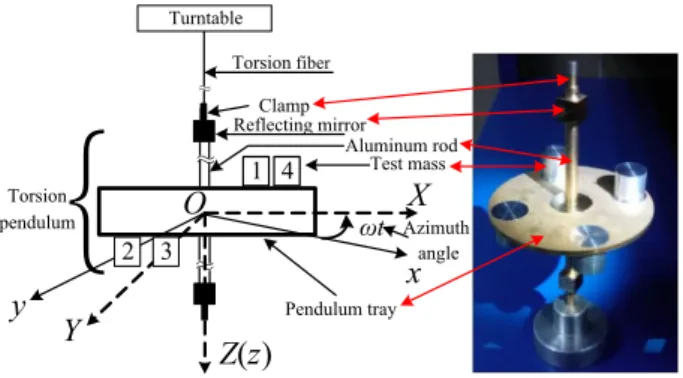
As the Fig.1shows, our specific torsion pendulum consists of four identical cylindrical test masses made of aluminum (diameter: 15.50 mm, height: 13.42 mm, mass: 2.53 g), with essentially the same mass. They are positioned on a circular aluminum pendulum tray (diameter: 80 mm, thickness: 2.5 mm, mass: 33.93 g). The masses 1 and 4 marked as the black circles in Fig.1are above the tray, the masses 2 and 3 marked as the black dashed circles are under the tray, and the four masses form a square with the side lengths. The selection of arrangement for four test masses is beneficial for us to ensure the pendulum’s sensitivity of theWxzandWyz. We define a clear relation between the lab frame (O-xyz) and the rotating frame (O-XYZ) in order to describe the principle of the dynamic modu- lation explicitly. Both originsOof the above two frames are at the same center-of-mass of
Fig. 1 Schematic drawing of the pendulum tray, the four test masses and the autocollimator viewing from the top. The sequals 42.23 mm. Both origins Oof the above two frames are at the same center-of-mass of the torsion pendulum. Thex(X) and y(Y) are axes of the lab (rotating) frame. TheXandYare along the direction of test masses 2?1 and 1?4 respectively. The xandyare towards East and North respectively
the torsion pendulum which rotates with the turntable together. TheX-axis andY-axis of the rotating frame (O-XYZ) are always along the directions of mass 2 pointing to mass 1 and mass 1 pointing to mass 4, respectively. The vertical axeszandZcoincide with the direction along the torsion fiber marked as the black line in Fig.2, parallel to the net force on the pendulum. The horizontal axes of the lab frame,xandy, are parallel to North and East respectively in geodesy. As the Fig.2shows, in our dynamic modulation measure- ment, we adjust the two frames to coincide with each other when the pendulum is in the equilibrium position, which occurs before we start to measure the gravity gradients. Then, we keep the pendulum rotating with the turntable at a constant angular velocityx. Thetis the dynamic modulation time, and the azimuth anglextis the rotation angle of the rotating frame relative to the fixed lab frame in the dynamic modulation. The deflection angle h(t) of the pendulum is measured in rotating frame by an autocollimator which rotates together with the pendulum counterclockwise.
The inertia tensors of the pendulum, ILM(L,M=X, Y,Z) can be calculated by the physical parameter of the pendulum in theO-XYZ, and they are constant because both of the pendulum and the rotating frame rotate together with the turntable. In other words, the relative position between pendulum and the rotating frame is constant.
The torque about the fibers(t) caused by the gravity gradients on the whole pendulum is (Vo¨lgyesi2015)
sðtÞ ¼ ðIYYIXXÞ WXYþIXZWYZ; ð3Þ whereWXY,WXZare gravity gradient components defined in theO-XYZ. TheWXYandWXZ
are just intermediate physical quantities and change in the different azimuth angle. These time-varying gravity gradient components should be converted into some gravity gradient components which are defined in fixed lab frameO-xyz. The relation between two frames is written as
Fig. 2 (color online) Schematic drawing of the torsion pendulum, viewing from the front. The schematic drawing correspond to the photo of the pendulum. The torsion fiber and the two frames we defined are shown. The torsion pendulum consists of the two same clamps denoted as the black rectangles, two reflecting mirrors marked as theblack squares, two same aluminum rods, four same test masses marked as therectangle frameand a pendulum tray shown as theblack rectangle frame. Theblack full lineis the torsion fiber. The two frames are marked as theblack solidanddashed lineswitharrows, respectively. The azimuth angle between the two frames is marked as thext
X¼xcosðxtÞ þysinðxtÞ Y¼ycosðxtÞ xsinðxtÞ Z¼z
8<
: : ð4Þ
Then Eq. (3) can be rewritten as:
sðtÞ ¼ ðIYYIXXÞsinð2xtÞ=2 ðWyyWxxÞ þ ðIYYIXXÞcosð2xtÞ Wxy
þIXZðcosðxtÞ WyzsinðxtÞ WxzÞ; ð5Þ whereWxx,Wyy,Wxy,WxzandWyzare gravity gradients defined in theO-xyz. The pendulum has a tiny deflection angleh(t) under the torques(t), and the torque is expressed as:
sðtÞ ¼khðtÞ; ð6Þ
wherekis the torsional spring constant of the fiber (Tu et al.2010).
In this way, we could observe the h(t) to obtain the torque about the fiber, and then measure the gravity gradient components defined in the O-xyz. The observed deflection angle of the pendulum is expressed as:
hðtÞ ¼ ðIYYIXXÞðWyyWxxÞsinð2xtÞ
ð2kÞ þ ðIYYIXXÞWxycosð2xtÞ k þIXZðcosðxtÞWyzsinðxtÞWxzÞ
k: ð7Þ
Equation (7) shows that theh(t) is a sinusoidal function of the turntable rotation angle xt. And theh(t) consisting of 1x, 2xorthogonal signals with four coefficients of the sine signal amplitude components a1sin, a2sin equals -(IXZ/k)Wxz and ((IYY-IXX)/
(2k))(Wyy-Wxx), respectively. The cosine signal amplitude componentsa1cos,a2cosequals (IXZ/k)Wyz and ((IYY-IXX)/k)Wxy, respectively. For every cycle of rotation, we can estimatea1sin,a1cos,a2sinanda2cosaccurately via the nonlinear least-squaring fitting method.
Then, the three gravity gradient componentsWxy,WyzandWxz, and the linear combination of the independent components (Wyy-Wxx) are given by:
WyyWxx¼2k=ðIYYIXXÞasin2 Wxy¼k=ðIYYIXXÞacos2 Wyz¼ ðk=IXZÞacos1 Wxz¼ ðk=IXZÞasin1 8>
><
>>
:
: ð8Þ
For the traditional torque type gradiometer with the static operating mode, thehis not a consecutive sinusoidal signal but five discrete data. The discrete data obtained from the observation of thehat five difference azimuth angles (Lancaster-Jones1932). Typically, this gradiometer sets the torsion pendulum at 0, 72, 144, 216, 288azimuth angles and then observehfor each azimuth angle (Shaw and Lancaster-Jones1922; Vo¨lgyesi2015).
In this way, observers could calculate the four gravity gradient components (Wyy-Wxx), Wxy,Wyz andWxzby the five independent equations based on Eq. (7). In this operating process, observers alternate azimuth angles of the pendulum regularly, and then the pen- dulum starts to swing. The torsion pendulum has a period of swing exceeding 20 min, and after having been disturbed returns to rest in its almost equilibrium position in approxi- mately 2 h (Shaw and Lancaster-Jones 1922). Besides, the h is recorded only after the torsion pendulum at a almost steady state. Therefore, most of the observe time is used to wait for the pendulum reaching to its equilibrium position, and it needs a complete observe cycle of at least 12 h.
For the improved gradiometer with dynamic modulation, as above mentioned, theh(t) is modulated as a sinusoidal signal by the rotating turntable. The recorded h(t) is a real reflection of the external torque coming from the gravity gradients, and the signal is sampled from the deflection angle of the pendulum at uniformly-spaced azimuth angles continuously during the experiment. That is to say, the improved gradiometer increase the sampling rate, and then decrease the observing time. It avoids costing much time as the traditional torque type gradiometer does. For every observed cycle, it could obtain a periodic signal which consists of 1xand 2xsine and cosine signals just as Eq. (7) shows.
Therefore, the four gravity gradient components can also be extracted from these sampled sinusoidal signals. The most distinct feature of the dynamic modulation measurement is that it needs less measurement time than the static operating mode. In this way, we could minimize the external fluctuations and improve the measurement accuracy. Besides, we can select a suitable rotation rate to avoid 1xor 2xsignals mixing with the free torsion oscillation signal of the pendulum.
3 Description of the gradiometer
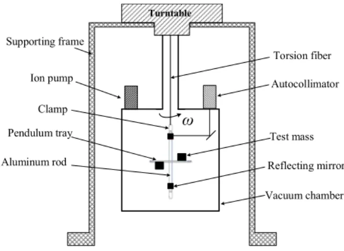
The scheme of the experimental apparatus used to perform the measurements is shown in Fig.3. The main body of the torsion pendulum is suspended by an annealed tungsten fiber (Goodfellow Cambridge Limited) with a length of 1000 mm and a diameter of 25lm, which hangs from a clamp which connects with an aluminum rod (long: 110 mm, diam- eter: 6 mm, mass: 2.67 g). And the aluminum rod is through the center of the pendulum tray, and two reflecting mirrors and two clamps are installed on its bottom and top sym- metrically. The total mass of the torsion pendulum equals 73.35 g which is a half of the max load of the fiber, and hence the fiber is maintained safe working status during the experiment. The top of the tungsten fiber connects to the vacuum chamber marked as the thick black full line in Fig.3, which is fixed on the turntable. The turntable is driven by a stepper motor and fixed on a supporting frame. An ion pump, which locates on the vacuum chamber and rotates with the turntable, is used to maintain a pressure of*10-5Pa (SP- 400) in the chamber during the experiments. Then the air damping can be negligible. An autocollimator (ELCOMAT 3000), which also locates on the vacuum chamber and rotates
Fig. 3 A front view of the improved gradiometer in our measurement. The pendulum, ion pump, autocollimator and torsion pendulum rotate together at a constant angular velocityx
with the turntable, is used to measure the deflection angleh(t) of the torsion pendulum. The inertia tensors of the pendulum are calculated in theO-XYZ, and theIXX,IYY,IXZandIZZare 45.404, 45.404, 4.620 and 52.822 kg mm2 respectively. This installation leads to IXX=IYY, so we can measureWxz,Wyzbased on Eq. (8) at present.
We divide the experiment into 4 steps. For the first step, we use the rotary vane pump, the turbo molecular pump and an ion pump to maintain a pressure of 10-5 Pa in the chamber during the experiment. For the second step, we let the two frames coincide when the pendulum is in the equilibrium position before formal measurement of the gravity gradients by adjusting the fiber. For the third step, the rotation period T of the turntable drive motor is set 1200 s, then the turntable drive motor is activated, and thus pendulum starts to rotate around theZaxis slowly. Meanwhile, the rotating autocollimator records the discrete data of the deflection angleh(t) at a regular interval of 1 s. Finally, we obtain a angle-time data set {h(ti),i=1,2,…}, wheretiis the sequence of sampling time.
4 Systematic effects
Thermal noise is one of the most fundamental limits to the precision of mechanical measurements, which is also of great importance and needs considering in the high- sensitivity gradiometer. Besides, in the improved gradiometer, since we use the turntable which rotates continuously at a constant velocity during the observation, we should also consider the effect from the irregular rotation rate of the turntable on the gravity gradients.
4.1 Thermal noise
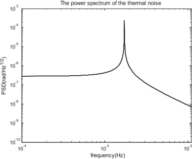
Thermal noise originates from Brownian motion, and the power spectrum of theh(t) due to the thermal noise could be written as:
jhðxÞj2¼ 4kBTI~ZZx0Q
ðkIZZx2Þ2Q2þIZZ2 x2x20; ð9Þ wherekB,T~andQare Boltzmann constant, ambient temperature and quality factor of the torsion balance system, respectively (Saulson1990). And the resonant frequencyx0equals
ffiffiffiffiffiffiffiffiffiffiffi k=IZZ
p . In our experiment, theQof the fiber approximates to 3000, theT~approximates to 294 K, thekequals 6.2910-9Nm/rad and the corresponding x0is about 0.0108 rad/s.
We plot the thermal noise power spectrum of theh(t) in Fig.4.
If the measuring frequency ranges from 0 to 0.001 Hz, then thermal noise limit can be expressed as:
dTnoisepotentialh¼
ffiffiffiffiffiffiffiffiffiffiffiffiffiffiffiffiffiffiffiffiffiffiffiffiffiffiffiffiffiffiffiffiffiffiffi Z 0:001Hz
0
hðfÞ j j2df s
¼1:18e8rad: ð10Þ
According to the principle of the error average distribution (Kirkup and Frenkel2006) dTnoiseasin1 ¼dTnoiseacos1 ¼dTnoisepotentialh= ffiffiffi
2
p ; ð11Þ
where dT-noisea1sin and dT-noisea1cos are the errors of the thermal noise on a1sin and a1cos respectively. From Eq. (8), the errors of the thermal noise toWxzandWyxis given as:
dTnoiseWxz¼ k IXZ
dTnoiseasin1
dTnoiseWyz¼ k IXZ
dTnoiseacos1 8>
><
>>
:
: ð12Þ
As a result, our gradiometer measurement resolution forWxzandWyxare both 0.01 E based on Eqs. (10–12).
4.2 Irregularities in the rotation rate
Suppose that the rotation of the turntable is not uniform, but it can be modulated at the rotation frequencyx and/or its higher harmonicsnx. Then the actual turntable rotation angleais expressed as:
a¼xtþX1
n¼1
Uneinxt;
whereUnare complex numbers. The deflection angle of the pendulum in the lab frame is defined ashL(t) (Su1992; Choi2006). Here the external torque is zero and the damping is ignored, and then the equation of the pendulum motion can be further written as (Su1992):
IZZh€L¼ kðhLaÞ ¼ k hLxtX1
n¼1Uneinxt
: ð13Þ
10-4 10-3 10-2
10-10 10-9 10-8 10-7 10-6 10-5 10-4 10-3
The power spectrum of the thermal noise
frequency(Hz) PSD(rad/Hz1/2)
Fig. 4 The power spectrum of the thermal noise.The horizontal axisandvertical axisare the frequency and the amplitude of the power spectrum of the thermal noise
The solution of Eq. (13) is
hL¼xtþX1
n¼1
x20
x20n2x2Uneinxt:
Therefore, in the rotating frame, the deflection anglehis converted into:
h¼hLa¼X1
n¼1
n2x2
x20n2x2Uneinxt: ð14Þ Ifnequals 1, then there is a spurious 1xsignal due to the irregularities in the rotation rate. The coefficients of the sin and cosine components are given by
dturntableasin1 ¼ x2
x20x2U1; dturntableacos1 ¼ x2
x20x2U1 ð15Þ The deviationsdturntableWxzanddturntableWyzof theWxzandWyzdue to irregularities in the rotation rate effect are expressed as:
dturntableWxz¼ k IXZ
dturntableasin1
dturntableWyz¼ k IXZ
dturntableacos1 8>
><
>>
:
; ð16Þ
It is necessary that the rotation rate of the turntable should be controlled at a single rotation frequencyx.Typically, all of the complex numbers |Un| are less 0.1lrad, and then the deviations of theWxzandWyxdue to irregularities in the rotation rate are 0.03 E based on Eqs. (15,16).
5 Experiment result
Before the formal measurement, we consider the measuring range of the improved gra- diometer (Vo¨lgyesi and Ultmann 2012), but we do not find a point where the gravity gradients are big value in our lab. Since the range depends crucially on the measuring range of the autocollimator (ELCOMAT 3000), the range, namely the maximum mea- surable angle of theh(t), of the ELCOMAT 3000 we adopted is±14,059.6lrad (±290000).
According to the Eq. (8) e.g.
ffiffiffiffiffiffiffiffiffiffiffiffiffiffiffiffiffiffiffiffiffiffiffiffiffiffiffiffiffiffiffi ðacos1 Þ2þ ðasin1 Þ2 q
14059:6lrad, the measuring range of the gradiometer is limited by an in equation ffiffiffiffiffiffiffiffiffiffiffiffiffiffiffiffiffiffiffiffi
Wxz2 þWyz2
q 18873:4E. It concludes that the gradiometer can measureWxzandWyzof a point where both of |Wxz| and |Wyz| are smaller than 13300 E.
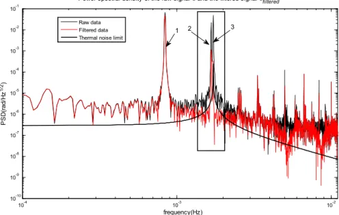
After about forty-four hours formal measurement with the improved gradiometer, we obtain the angular deflection h(t) of the torsion pendulum shown in Fig.5. We find that h(t) is not a simple sine (or cosine) signal, and it contains other frequency signals. Then, we plot the spectrum of the whole raw data shown in Fig.5. We find that there are 1x, 2xand x0signals in the raw data. The 1xsignal is the useful oscillation signal for us to obtainWxz
andWyz. The 2xsignal is the second harmonic of the useful oscillation signal, caused by the defective of the pendulum(the inertia tensorsIXXandIYYare not equal strictly) and the
20 20.5 21 21.5 22 22.5 23 -5
0 5 10 15x 10-4
Time(hours)
Amplitude(rad)
The deflection angle θ(t) of the pendulum
(a)
5 10 15 20 25 30 35 40
-5 0 5 10 15x 10-4
Time(hours)
Amplitude(rad)
The deflection angle θ(t) of the pendulum
(b)
Fig. 5 The raw datah(t) from 44 h (about 130 turntable periods) of a normal experiment. Theblack lineis the signalh(t).aThe angular deflectionh(t) of the pendulum versus time at the time from 20 to 23 h;bThe angular deflectionh(t) of the pendulum versus time during the whole measurement. Thehorizontal axisis the sampled time series, and thevertical axisis the amplitude of theh(t)
10-2.8 10-2.7
10-8 10-7 10-6 10-5 10-4 10-3 10-2 10-1
frequency(Hz) PSD(rad/Hz1/2)
The power spectrum of the thermal noise
Raw data Filtered data Thermal noise limit
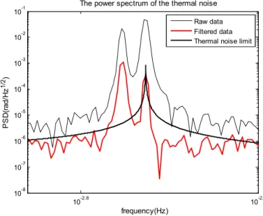
Fig. 6 (color online) The enlarged drawing of theblack framein Fig.7
irregularities in the rotation rate (in the Eq. (15), let n equals 2). We could use a very symmetrical pendulum and keep rotation rate steady to suppress the 2xsignal if we need the improved gradiometer to obtain a higher measurement precision. Thex0signal is the free torsion oscillation signal caused by the physical characteristic of the torsion fiber.
As the Fig.6show, we could use the frequency estimation method (Quinn 1994) to extract the period of the free torsional oscillation signalT0. And then, we estimate theWxz
andWyzby the following 5 steps of the data processing.
Firstly, we use a torsional filter (Su1992) to process the raw data in order to eliminate the x0 signal. The torsional filter is to add two data points separated by p of torsional phase, expressed as
hfilteredðtÞ ¼1
2 h tT0
4
þh tþT0
4
;
whereT0 is the period of the free torsional oscillation signal and equals 579.9 s in our experiment. Then, the filtered signalhfiltered(t) equals {hfiltered(ti)}. In this way, the torsional oscillation signal will be significantly minimized in raw data. Meanwhile, the useful amplitude of the 1x signal has also be attenuated by a factor R(x)=cos(xT0/4) (Su 1992), and in our experiment, theR(x) of the 1xsignal is about 0.72. This attenuation needs to be corrected for the 1x signal in result. The power spectral density of the amplitude of the filter data shows in Fig.7. We find that the x0 signal is decreased by about two orders, and the filtered 2xsignal is reduced to about the 1/25 of the raw 2x signal at the same time. The amplitude attenuation of the useful 1xsignal can be corrected to real amplitude in result. The data, which is usually two day long, has a irregular drift in
10-4 10-3 10-2
10-10 10-9 10-8 10-7 10-6 10-5 10-4 10-3 10-2 10-1
frequency(Hz) PSD(rad/Hz1/2)
Power spectral density of the raw signal θ and the filtered signal θfiltered
Raw data Filtered data Thermal noise limit
1 2 3
Fig. 7 (color online) Power spectral density of the raw signalhand the filtered signalhfiltered. Theblue,red andblack linesdenote the power spectral densities of the raw signal, filtered signal and thermal noise, respectively. The peaks 1, 2 and 3 marks 1x, 2xandx0signal, respectively. Thehorizontal axisis the frequency, and thevertical axisis the amplitude. The details of the PSD between peak 2 and 3 are encircled by ablack rectangleframe which shown in Fig.6
temperature. Although this drift is small, its effect can be reduced by cutting the entire data into smaller segments and fitting each separately.
Secondly, each segment contains 3 periods of turntable, and then the filtered data is divided into 43 segments in the experiment. For the jth segment, the filtered data is fhfilteredj ðtiÞgi¼1;2;;3Tj¼1;2;...;43, then the cut angular deflection signalhc
j(t) in thejth segment could be express as
hcutj ðtÞ ¼ fhfilteredj ðtiÞgi¼1;2;...;3600 j¼1;2;...;43 :
Because each segment consists of an integer number of cycles, the harmonic terms in fit function are orthogonal to each other. The reason that we do not use shorter cuts is to ensure the harmonic terms approximately orthogonal to the drift terms and to have enough data points for a reliable fit (Choi2006).
Thirdly, for every segment, we use the nonlinear least-squaring fitting method to fit the filtered signal points to extract the sine and cosine amplitude components of themxsignal in the jth segment. A similar nonlinear fitting method has been used in testing the equivalence principle by Gundlach et al. (1997). Base on the signal component of the experimental data, the goal fitted function could be written:
h^cjðtÞ ¼bjþcjtþXh
m¼1
ðacosm;jcosðmxtÞ þasinm;jsinðmxtÞÞ;
wherebjis constant term,cjis liner drift coefficient,mdenotes themorder harmonic of the useful signal and the highest itemhis set 9, and (asinm;j,acosm;j) is the (sine, cosine) amplitude
0 5 10 15 20 25 30 35 40 45
64.2 64.4 64.6 64.8
j
Amplitude(urad)
The cosine amplitude component of the 1ω signal in jth cut data
(b)
0 5 10 15 20 25 30 35 40 45
326 326.5 327 327.5
j
Amplitude(urad)
The sine amplitude component of the 1ω signal in jth cut data
(a)
Fig. 8 The blank pointsare fitting value of the 1xsignal component coefficient in every segment. The
components of themxsignal in thejth segment (j=1, 2,…, 43), respectively. We use this function because the filtered data has not significant drift or has only linear drift which is removed by the torsional filter.
Later, we use the Chi Square to test our fitting result:
v2j ¼ 1 r2i
X3600
i¼1
½ðhcutj ðtiÞ h^cutj ðtiÞ2;
where hcutj ðtiÞ is the jth segment of the filtered data, h^cutj ðtiÞ is our fitting result for jth segment filtered data. Theri2is every point standard deviation in thejth segment filtered data and we let riequals 0.5 lrad in our data process, the freedoms of the jth segment filtered datamequals 3580. Ifvj2[1, then we consider that theh^cutj ðtiÞis not fithcutj ðtiÞand it should be eliminated. In our experimental data that all 43 segments have been fitted eligible.
For thejth segment, the estimated value of the amplitude components, (asin1;j,acos1;j) are given by the above fitting accurately. These fitted amplitude components, {(asin1;j,acos1;j), j=1, 2,…, 43} should be corrected to the real amplitude components, {(~asin1;j,~acos1;j),j=1, 2,…, 43} base on Eq. (17).
~
asin1;j¼asin1;j=RðxÞ; a~cos1;j ¼acos1;j=RðxÞ: ð17Þ
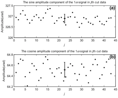
Then, the corrected amplitude of the components is plotted in Fig.8.
The average values, (asin1 ,acos1 ) and error bars, (rasin1 ,racos1 ) of the 1xsignal component coefficient could be obtained by statistical and average for the {(~asin1;j,~acos1;j), j=1, 2,…, 43}:
asin1 ¼ 1
43 X43
j¼1
~
asin1;j; rasin1 ¼
ffiffiffiffiffiffiffiffiffiffiffiffiffiffiffiffiffiffiffiffiffiffiffiffiffiffiffiffiffiffiffiffiffiffiffiffiffiffiffiffiffiffiffiffiffiffiffiffiffiffiffiffiffiffiffi 1
43ð431Þ X43
j¼1
ð~asin1;jasin1 Þ2 vu
ut ; ð18Þ
acos1 ¼ 1
43 X43
j¼1
~
acos1;j; racos1 ¼
ffiffiffiffiffiffiffiffiffiffiffiffiffiffiffiffiffiffiffiffiffiffiffiffiffiffiffiffiffiffiffiffiffiffiffiffiffiffiffiffiffiffiffiffiffiffiffiffiffiffiffiffiffiffiffiffi 1
43ð431Þ X43
j¼1
ð~acos1;j acos1 Þ2 vu
ut : ð19Þ
Base on Eqs. (18) and (19), the result of the average value and the error bars could be written:
asin1 ¼ ð326:890:03Þlrad acos1 ¼ ð64:520:02Þlrad (
:
The measurement results of the each segment are coincide within the error bar.
According to Eq. (8), the measurement result of theWxzandWyzcould be shown:
Wxz¼ ð438:680:04ÞE Wyz¼ ð86:580:03ÞE (
:
For the whole experiment, the measurement accuracyrWxzandrWyzof theWxzandWyz
are 0.04 E and 0.03 E respectively. We usually use a period of the turntable to complete a single measurement, and then the single measurement accuracy r1Wxzandr1WyzofWxz
andWyzcould be show in Eq. (20)
r1Wxz¼ ffiffiffiffiffiffiffiffiffiffiffiffiffiffi 343 p rWxz r1Wyz¼ ffiffiffiffiffiffiffiffiffiffiffiffiffiffi
343 p rWyz
(
; ð20Þ
where 3943 is the number of the periods for the whole experiment.
The single measurement accuracyr1Wxzandr1Wyzof the improved gradiometer will extend to 0.45 E and 0.32 E respectively based on Eq. (20).
6 Comparative measurement
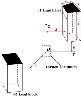
In order to the practical justification of the theoretical considerations, we develop an independent comparative measurement (Vo¨lgyesi and Ultmann 2012; Vo¨lgyesi 2015) before the formal measurement. As the Fig.9 shows, we structure a calculable and knowable gravity gradient fieldGGbby installing two lead blocks around the pendulum, and then test the responses (sensitivity) of the improved gradiometer to the artificial field GGb. According to Eq. (5), we could only consider the deflection angleh(t) of the pen- dulum at the frequency 1x. In this way, we perform the comparative measurement by three steps. Step 1: we spend 15 h measuring theh(t) of the torsion pendulum in the fieldGG0 without setting the blocks, and the gravity gradient field is uniform and even. Step 2: we measure theh(t) of the torsion pendulum in the field with setting the blocks about 9 h, and this field is marked as GG0?GGb. Step 3, we remove the lead blocks and remeasure h(t) in the gravity gradient fieldGG0.
Torsion pendulum
#1 Lead block
#2 Lead block
a w b
h
x
y z
O H
R
Fig. 9 (color online) Schematic drawing of the lead blocks and the pendulum. The #1 and #2 lead block are essentially the same blocks. The two blocks are symmetric about the origin of the lab frame (O-xyz). The cross-section of the block is isosceles trapezoid. The upper and lower side lengtha, band the height of the trapezoidw are equal to 9.39(5), 11.89(5) and 7.9(1)cm, respectively. The height of the block equals
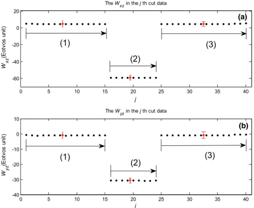
We measure theh(t) of the torsion pendulum in the fieldsGG0,GG0?GGbandGG0 orderly. As the Fig.10shows, we obtainedWxzandWyzof the fieldGG0 with the same method we adopt in formal measurement. Then we use the spherical function expansion (Su 1992; Landau 2013) to calculate out the standardized 21th order multipole field Qb21¼ ½156ð1Þ i73ð3Þ 109=s2of theGGb, and further the theoreticalWxzb andWyzb duo to the fieldGGb. And the relation between theQb21 and theWxzb,Wyzb is (Landau2013):
0 5 10 15 20 25 30 35 40
-40 -30 -20 -10 0 10
j W yz(Eotvos unit)
The Wyz in the j th cut data
0 5 10 15 20 25 30 35 40
-60 -40 -20 0 20
j W xz(Eotvos unit)
The Wxz in the j th cut data
(3) (2)
(1) (2) (1)
(3)
(a)
(b)
Fig. 10 (color online) Theblank pointsare the fitting values of theWxzandWyzin every segment. Thered asteriskand itserror bardenote the final value and uncertainty of the corrected value, respectively. The number (1), (2) and (3) are labeled as the fieldsGG0,GG0?GGbandGG0, separately. There are 15, 9 and 16 sets of (Wxz,Wyz) in the fieldsGG0,GG0?GGlbandGG0, respectively.a: TheWxzin thejth cut data.b:
TheWyzin thejth cut data
Table 1 The result of the independent comparative measurement and its corresponding theoretical value Gravity gradient field Wxz(theoretical) Wyz(theoretical) Wxz(measured) Wyz(measured)
Step 1 GG0 – – -4.61 (6) -0.84 (5)
Step 2 GG0?GGb – – 59.12 (4) -30.73 (1)
Step 3 GG0 – – -4.56 (4) -0.91 (3)
GGb 63.69 (5) -29.83 (4) 63.70 (8) -29.85 (6)
Qb21¼ 1 ffiffiffi6
p Wxzb þiWyzb
: ð21Þ
With the same way we use in formal measurement, the result of the independent comparative measurement could be summarized in Table1.
As the Table1shows, on the one hand the single measurement accuracies of the Steps 1–3 and the formal measurement are in good agreement. On the other hand, the mea- surement results of the Steps 1 and 3 are still in good agreement. That is to say, the measurement accuracy of the improved gradiometer is consistent. We can calculate the measuredWxzandWyzof the fieldGGbfrom the results of the Steps 1–3, and the measured WxzandWyz are agree with the theoretical value. It is mean that the gradiometer could response the artificial fieldGGbcorrectly. Therefore, the independent comparative mea- surement indicate that the measurement of the improved gradiometer is stable and effective.
7 Conclusions
In the measurement of the gravity gradients with the traditional torque type gradiometer, it is of inefficiency and with relatively low accuracy due to the static operating mode. To improve the efficiency and accuracy, we develop an improved torque type gradiometer by using dynamic modulation mode. In the dynamic modulation mode, the torsion pendulum is mounted on a continuously rotating turntable with a constant rate, and the gravity gradients are extracted from the deflection angle signal that is modulated by the turntable.
This improvement shortens the measurement cycle largely and improves the accuracy of the obtained gravity gradients effectively. The experimental results show that at the same accuracy of 1 E, the measurement cycle of the improved torque type gradiometer is only about one thirty-sixth of the traditional gradiometer. In the measurement of the gravity gradient by the improved torque type gradiometer with dynamic modulation, the uncer- tainties of the obtained gravity gradient componentsWxzandWyzare 0.45 E and 0.32 E respectively, which are more precise than those obtained by the traditional torque type gradiometer. The results of independent comparative measurement show that the mea- surement of the improved gradiometer is stable and effective. The errors of the thermal noise on the gravity gradient components Wxz and Wyz are 0.01 E. The errors of the irregularities in the rotation rate on the gravity gradient componentsWxzandWyzare 0.03 E. The improved torque type gradiometer with dynamic modulation is highly efficient and accurate. Because of the short measurement cycle, the observation can avoid many noises and disturbances from external environment, and hence this improved torque type gra- diometer may have a wide potential in practical applications. Besides, due to the config- uration of our instrument and the particular positions of the four test mass, the preliminary experiment of the gravity gradient with our improved gradiometer determines two com- ponentsWxzandWyzof the gravity gradient. As long as we alter the positions of the four test mass, our improved gradiometer can also obtain the four components of the gravity gradient like the traditional gradiometer. It is instructive and significant to improve the torque type gradiometer measuring the gravity gradient. Since the gradiometer is a field device that must operate in the field condition and the carrying and working conditions in
some more improvement can be performed, our improved gradiometer can be used to engineering application promisingly. Since the configuration of the instrument and the position of test mass are not fully understood, there are still many works needed per- forming in the future.
Acknowledgements This work is partially supported by the National Natural Science Foundation of China (Grant Nos. 11575160, 91636221, 11605065).
References
Barton DC (1931) Gravity measurements with the Eotvos torsion balance. Consulting Geologist and Geophysicist, Houston, Texas. Physics of the Earth 77:167–188
Bell RE, Hansen RO (1998) The rise and fall of early oil field technology: the torsion balance gradiometer.
Lead Edge 17(1):81–83
Choi KY (2006) A new equivalence principle test using a rotating torsion balance. Ph.D Dehlinger P (1978) Marine gravity, vol 22. Elsevier, Amsterdam
DiFrancesco D, Grierson A, Kaputa D, Meyer T (2009) Gravity gradiometer systems—advances and challenges. Geophys Prospect 57(4):615–623
ELCOMAT 3000, Germany Moeller-Wedel Optical GmbH.https://www.haag-streit.com/de/moeller-wedel- optical/
Goodfellow Cambridge Limited, Huntingdon PE29 6WR, England.http://www.goodfellow.com/contact-us/
Gundlach JH, Smith GL, Adelberger EG, Heckel BR, Swanson HE (1997) Short-range test of the equiv- alence principle. Phys Rev Lett 78(13):2523
Kirkup L, Frenkel RB (2006) An introduction to uncertainty in measurement: using the GUM (guide to the expression of uncertainty in measurement). Cambridge University Press, Cambridge
Lancaster-Jones E (1932) The principles and practice of the gravity gradiometer. J Sci Instrum 9(11):341 Landau LD (ed.) (2013) The classical theory of fields, vol 2. Elsevier, Amsterdam
Luo J, Shao CG, Tian Y, Wang DH (2013) Thermal noise limit in measuring the gravitational constant G using the angular acceleration method and the dynamic deflection method. Phys Lett A 377(21):1397–1401
Quinn BG (1994) Estimating frequency by interpolation using Fourier coefficients. IEEE Trans Signal Process 42(5):1264–1268
Rankine AO (1932) On the representation and calculation of the results of gravity surveys with torsion balances. Proc Phys Soc 44(4):465
Saulson PR (1990) Thermal noise in mechanical experiments. Phys Rev D 42(8):2437
Schweydar W (1918) Die Bedeutung der Drehwaage von Eo¨tvo¨s fu¨r die geologische Forschung nebst Mitteilung der Ergebnisse einiger Messungen. Zeitschrift fu¨r praktische Geologie 26:157–162 Shaw H, Lancaster-Jones E (1922) The Eo¨tvo¨s torsion balance. Proc Phys Soc Lond 35(1):151 SP-400, Shanghai Shanjin Vacuum Equipment Co., Ltd., Shanghai, China
Su Y (1992) A new test of the weak equivalence principle. Ph.D
Szabo´ Z (2016) The history of the 125 year old Eo¨tvo¨s torsion balance. Acta Geod Geoph 51(2):273–293 Tu LC, Li Q, Wang QL, Shao CG, Yang SQ, Liu LX, Liu Q, Luo J (2010) New determination of the
gravitational constant G with time-of-swing method. Phys Rev D 82(2):022001
Vo¨lgyesi L (2001) Local geoid determination based on gravity gradients. Acta Geodaetica et Geophysica Hungarica 36(2):153–162
Vo¨lgyesi L (2015) Renaissance of torsion balance measurements in Hungary. Periodica Polytechnica Civ Eng 59(4):459
Vo¨lgyesi L, Ultmann Z (2012) Reconstruction of a torsion balance and the results of the test measurements.
In: Kenyon SC, Pacino MC, Marti UJ (eds) Geodesy for planet earth. Springer, Berlin, pp 281–289 Zhou MK, Duan XC, Chen LL, Luo Q, Xu YY, Hu ZK (2015) Micro-Gal level gravity measurements with
cold atom interferometry. Chin Phys B 24(5):050401