Development of Complex Curricula for Molecular Bionics and Infobionics Programs within a consortial* framework**
Consortium leader
PETER PAZMANY CATHOLIC UNIVERSITY
Consortium members
SEMMELWEIS UNIVERSITY, DIALOG CAMPUS PUBLISHER
The Project has been realised with the support of the European Union and has been co-financed by the European Social Fund ***
**Molekuláris bionika és Infobionika Szakok tananyagának komplex fejlesztése konzorciumi keretben
***A projekt az Európai Unió támogatásával, az Európai Szociális Alap társfinanszírozásával valósul meg.
PETER PAZMANY CATHOLIC UNIVERSITY
SEMMELWEIS UNIVERSITY
Peter Pazmany Catholic University Faculty of Information Technology
MODELLING NEURONS AND NETWORKS
Lecture 9
Models of memory
www.itk.ppke.hu
(Idegsejtek és neuronhálózatok modellezése)
(Memóriamodellek)
Szabolcs Káli
Overview
In this lesson you will learn about the structure and workings of the
neural networks responsible for storing and recalling memory traces. We will discuss several theories that try to explain how short- and long-term memory work.
Lesson topics:
•
Short-term memory
•
Recurrent network models of short-term memory
•
Model for working memory and decision making
•
Long-term memory: the hippocampus as a long-term memory store.
•
An attractor network model of spatial representations in area CA3
•
Generating non-directional place fields
•
The effects of manipulating the environment
•
Spatial representations, special cases: very different and very similar
environments
Short-term memory
• Can store only a few items at the same time.
• Can only store items for a limited amount of time. The cause of the decay is debated: Some suggest that its contents spontaneously degrade over time. Others explain the degradation by a competitive model: When many items are stored in memory, these elements compete with each other, so the more active content pushes out the less active ones.
• Persistent neural activity is required for the storage – excitatory synaptic loops could be responsible for it.
• Synaptic inhibition is also likely to be critical for shaping the selectivity of mnemonic neural activity in a working memory circuit.
• Studies have shown that when there is a delay between the
stimulus and the response, neurons show a selectively
enhanced activity throughout the delay period in the prefrontal
cortex (PFC) and in the inferotemporal cortex (ITC).
Recurrent network models of short-term (working) memory
Brunel and Wang, 2001: Model of object working memory in a large cortical network that is dominated by feedback inhibition. The model represents a cortical module of an area receiving information about the identity of objects.
Main features of the model:
• Persistent activity is generated within a local cortical circuit.
• Recurrent synaptic excitation is largely mediated by NMDA receptors.
• Recurrent network interactions are dominated by synaptic inhibition.
The network is composed of two types of cells: excitatory pyramidal cells (80% of the cells) and inhibitory interneurons (20%). Both are represented by integrate-and-fire models (see Lecture 7).
Both pyramidal cells and interneurons also receive excitatory connections
from outside the network. These connections send to the network all the
information (stimuli) received from the outside world, as well as
background noise due to spontaneous activity outside the module.
Recurrent network models of short-term (working) memory
Figure: Schematics of the memory model (explanation on next page).
Recurrent network models of short-term (working) memory
• Pyramidal cells send connections to other pyramidal cells and interneurons through AMPA and NMDA synapses.
• Interneurons send GABAergic connections to pyramidal cells and other interneurons.
• Both receive excitatory connections from other cortical areas.
• Pyramidal cells can be functionally divided in several groups
according to their selectivity properties. Group #1 is selective to
object #1, etc. Cells within a group have relatively stronger
connections (modulated by w+ > 1), while connections between
different groups are relatively weaker (modulated by w− < 1).
Delayed-match-to-sample task protocol
1. There is a 1 second startup period, in which the network exhibits spontaneous activity.
2. Stimulus presentation (sample) consists of a transient input (lasting for 500msec) to those cells selective to the shown stimulus. Other cells are unaffected.
3. After the external stimulus is removed, there is a delay period of 4 s.
4. Finally, a match stimulus is presented for 500ms. In the last
400ms of the match presentation, the external frequency to all
cells is multiplied by 1.5 to account for an increase in afferent
inputs due to the behavioral response/reward signal.
Delayed-match-to-sample task analysis
Figure: Network activity during the delayed- match-to-sample task.
A: Average activity of different types of cells.
Red: cells selective for the shown stimulus.
Green, yellow, blue, and brown: cells selective for other stimuli.
Cyan: cells not selective to any of the stimuli.
Black: Inhibitory cells.
The stimulus triggers persistent activity in a selective cell population (red) at about 25 Hz.
Delay period activity is switched off by a transient excitatory input generating a brief surge of activity in all neurons.
B: Interspike interval histograms of cells selective to the input sample during spontaneous and persistent activity.
Memory preservation in the presence of distractors
A distractor is a nonmatch stimulus different from the initial sample. It is applied to those neurons which are sensitive to this stimulus and with the same frequency as the sample and match stimuli.
The effect of distractors on network activity depends mainly on the stimulus amplitude (see figure in next page):
• At very weak stimulus intensity, presentation of the sample stimulus was unable to elicit any elevated delay activity.
• For intermediate values of stimulus amplitude the stimulus caused persistent activity that was resistant to distractors.
• For high values of stimulus amplitude, cue-related persistent activity (short- term memory) is disrupted by the nonmatch stimuli and the network is
distracted. In this case, a nonmatch stimulus is sufficiently powerful to bring its corresponding neuronal assembly (whose best stimulus is the distractor) from a low firing state to its high firing state. The initial match neural
population’s persistent activity is disrupted. These cells are turned off as a dynamical consequence of the rise of the new neuronal subpopulation, which leads to a transient surge of feedback inhibition to the rest of the network.
Results on the delayed-match-to-sample task
Figure A: The network retains its ability to recall the sample with
distractor stimuli at immediate intensities.
Figure B: The persistent activity is disturbed if the distractor intensity is high enough, and the network changes into another persistent state.
Red: initial stimulus population activity.
Green, violet: distractor population activity.
Combined model of working memory and decision-making
Machens, Romo, and Brody (2005): Model of working memory and decision making. The model’s main feature is mutual inhibition between the network units, which is a useful design motif of networks with multiple behaviors.
Experimental setup:
Stimuli are frequencies of vibrations applied to the tip of a monkey’s finger, and the activity of prefrontal cortical (PFC) and somatosensory cortical (S2) neurons is measured during the experiment.
1.Subjects perceive a short stimulus, called f1, and maintain it in their working memory.
2.They compare it after a delay with a brief second stimulus, called f2.
3.They decide immediately after which stimulus was larger.
Experimental setup and results
Horizontal scale indicates time, the rainbow colored bar indicates frequency for f1. For each trial, monkeys made the correct response more than 91% of the time.
A: Experiment setup. Stimuli are named f1 and f2.
B-E: Neuronal responses during the experiment. Blue lines at the end are „YES” responses; brown lines are „NO” responses. Color codes indicate f1 frequency during measurement.
B,C: Firing rates of prefrontal cortical (PFC) plus and minus neurons. The signals are encoded in two complementary sets of roughly equal number of neurons: Plus neurons (fig. B) fire the most if the decision at the end is „YES”, minus neurons (fig. C) if the decision is „NO”. During f1 (memorizing phase) and in the maintenance phase there is a strong f1-dependent firing rate.
During the comparison phase(f2), neurons segregate quickly into YES/NO categories. When the f1 stimulus is high, plus neurons tend to fire more, because „YES” answer is more likely, and the opposite is true for „NO” neurons. Each of the two sets carry all information necessary, the existence of redundant sets is unexplained.
D,E: Neuronal response in area S2. After 2.8 seconds, color codes indicate f2 response.
Model for working memory and decision making
One interesting finding of the experiments is that the same neurons which maintain the working memory are responsible for the decision making too.
The algorithmic representation for modeling both of these tasks:
•Both memory and decision making are represented by the value of a single state variable.
(dots on the picture, horizontal position indicates state variable value.)
•The dynamical modes are represented by an energy function L, the shape of which does not depend of the state variable. (line on the picture, energy levels are represented by the vertical axis.)
• The state variable always moves to a lower energy level.
• During the loading (memorizing) stage the external stimulus creates a single minimum in L.
• During the maintenance phase, there is no stimulus that determines the shape of L, thus L is flat.
• During the decision phase, the f2 stimulus is mapped onto a peak of the L function. Now all state positions to the left of the peak caused by f2 represent memories of a smaller f1, and vice versa.
If the horizontal axis stands for firing rate that grows from left to right, the position of the state variable mimics the firing rate of the plus neurons measured during the experiment. They mimic the minus neurons if the horizontal axis grows from right to left.
The authors of the article propose that the frontal-lobe areas instantiate this algorithm. Clues about the underlying architecture come from the analysis of firing-rate covariations between pairs of PFC neurons, which reveal distinct plus and minus neuron populations.
In a simplified version of this circuit each unit represents a population of neurons (fig. B), and the output is the average activity of the population. The response strength of these neurons to different strengths of excitatory input can be seen in fig. C (I/O function).
The dynamics of the circuit can be seen in Fig. D: The black line shows the output of the plus node as a function of the inhibitory output from the minus node (the plus node has a constant excitatory input applied.). The minus node’s I/O function is plotted by exchanging the horizontal and vertical axes (brown line).
This phase-plane plot describes the dynamics of the system. Points where the two curves intersect are steady-states, which can be stable of unstable.
Neural representation of the algorithm
Neural representation of the algorithm
Figure: Detailed explanation of the algorithm during storage (loading), maintenance and decision phase.
(for explanation see next page.)
Neural representation of the algorithm
(explanation of the figures on the previous page)
S2 plus neurons project to the PFC plus neurons, and S2 minus neurons project to the PFC minus neurons. Stimulus frequency in this figure corresponds to the angle of θ.
During the first stimulus, the position of the single stable point is determined by f1 (fig. E). Blue/green/red lines show the effect of three stimuli.
During the maintenance period inputs from S2 are silent (fig. F). The value of E (external constant input) can be chosen such that the two I/O curves largely overlap. This creates a continuous line of stable points.
During the decision phase (fig. G) it is assumed that E is externally reduced, to signal that the system is in the decision phase. Because E is low, there are two stable fixed points. Trajectories start from endpoints in fig. F.
In the experimental data, frontal neurons switch their stimulus dependence, but S2 neurons do not. This is represented by the circuit shown in fig. H.
As a result of this sign-switching, increasing f2 moves the unstable fixed point from a lower to a higher θ, which matches the f1-dependence of the stable point during loading.
Associative (long-term) memory
As we have seen, recurrent networks often have activity patterns which behave as fixed point attractors. These may also be considered as stored memory traces, provided that we can specify the fixed points (preferably via a plausible activity-based learning rule).
Auto-associative function: the dynamics of the network reconstructs the original pattern based on a fragment or a noisy version.
(Binary) Hopfield network:
• binary (-1 / +1) units
• all-to-all symmetrical connections
• linear threshold activation
• asynchronous state updates
• Hebbian learning
• dynamics minimizes energy function
• learning creates minima in the energy landscape
• learning multiple items can lead to spurious attractors
• capacity is about 0.14 N (N is the number of units)
Recurrent network models of long-term memory
The hippocampus as a long-term memory store
Capacity with graded-response neurons and sparse connectivity (model of hippocampal CA3 network by Treves and Rolls):
(1)
C
RCis the number of modifiable recurrent connections per cell, a is the
sparseness of individual patterns, k ~ 0.2 - 0.3.
If C
RC=12000 and a=0.02, p
max~36000.
More recent analysis with spiking neurons (Roudi and Latham, 2007):
P
maxis proportional to C
RCbut independent of a, p
max~120.
Two distinct modes of operation are needed:
• learning: plastic synapses, feedforward inputs dominating activity
• retrieval: no plasticity, strong recurrent interactions
May be implemented through neuromodulatory inputs (Hasselmo).
Two separate input pathways may be required:
• strong, sparse input during learning (mossy fibers)
• many associatively modifiable inputs for retrieval (perforant path)
The hippocampus as a long-term memory store
Spatial learning and memory depend on the hippocampus.
Place cells provide a population code for location (and other things).
How is this representation formed?
Does the CA3 recurrent network function as an attractor network in this case?
Samsonovich & McNaughton (1997): Fixed, statistically independent sets of attractors (continuous attractors) can be encoded.
But: experience-dependent, partially overlapping representations exist.
New idea: attractors may be determined by experience (in analogy with the fixed point attractors underlying memory for discrete items, as described earlier).
Formation of spatial representations in the hippocampus
Place fields:
•
compact, regular,
•
stable after ~10 minutes of exploration,
•
non-directional in open field,
•
directional in restricted environments.
•
"Orthogonal" representations for very different environments.
•
Entire set of place fields can follow transformations of the environment
•
Representations can overlap partially
Place cell representation
Place cell representation
Figure: place fields of five cells (recorded simultaneously).
The rat travels in a triangular maze; the dots indicate the locations where
each cell fired.
Model architecture
The model gets input from the entorhinal cortex (EC), whose activity is determined by the environment. This representation is transformed by feedforward pathways (direct input to CA3 and pathways through the dentate gyrus (DG)). The CA3 pyramidal cells (black circles) have recurrent connections and connections with inhibitory cells (open circles).
Solid lines represent connections that are modeled explicitly, solid thick lines represent modifiable connections.
The change of the membrane potential over time is described by the following equations:
Model dynamics
Where
ui is the membrane potential of the ith pyramidal cell,
v is the membrane potential of the global inhibitory cell (all relative to their resting potentials), and are the membrane time constants for pyramidal neurons and the inhibitory cell, respectively,
Jij is the strength of the connection from pyramidal neuron j to pyramidal neuron i, h is the efficacy of inhibition,
w represents the strength of the excitatory connection from any one pyramidal cell onto the inhibitory cell,
IiPP and IiMF are the inputs to cell i through the perforant path and the mossy fibers (MF), respectively.
gu(u)=[u-]+ is the threshold linear activation function for the pyramidal cells, where [. . .]+ makes all negative arguments zero but leaves positive numbers unaffected, stands for the threshold, and is the slope of the activation function above the threshold.
Sources of spatial information: all modalities Let us concentrate on:
• Visual inputs
• Self-motion - path integration
Inputs are location and direction dependent:
Model inputs
Left: The net two-dimensional tuning of a sample EC neuron in a rectangular box of dimensions 2x1; the preferred location of the cell is (0.5, 0.4); the current heading of the rat at each location is the same as the preferred head direction of the cell.
Right: The activity of an EC neuron as a function of the difference between its preferred direction and the actual heading of the rat.
Two-mode hypothesis (Hasselmo)
On-line neuromodulation of synaptic efficacies in the hippocampus by septal inputs (ACh and GABA).
Learning
(high ACh, in new environment)
• mossy fiber inputs dominate CA3 activity
• recurrent connections suppressed
• inhibition reduced
• plasticity in perforant path and recurrent synapses Recall
(low ACh, in familiar environment)
• recurrent connections dominate
• feedback inhibition
• plasticity suppressed
Inputs are directional, place fields in open environments are not - Can we account for this?
Generating non-directionality
1. Learning phase - establish weights
•
Assume equal exposure to all possible locations and head directions
•
Feedforward weights (perforant path) learn to represent essentially the same mapping from entorhinal cortex to CA3 as the pathway through the dentate gyrus
•
Recurrent weights determined by spatial correlations in DG inputs 2. Recall phase - run until convergence
•
CA3 place cell activity determined by attractor dynamics
•
Feedforward inputs select from attractors
When all headings are equally likely at each location during learning, the resulting attractors in the model can be direction independent.
Generating non-directionality
Figure: Population plots. Cells with a given preferred direction (north and south in this case) are arranged on an imaginary plane according to their preferred locations. This describes the behavior of all the cells with the actual position and heading of the animal kept fixed.
Plots show the activities of cells in EC, the net PP inputs to CA3 neurons (IiPP), and the final activities of the same place cells (marked CA3), as a function of the preferred location of the neuron; the two rows are for cells with preferred head direction indicated by the arrow next to each row.
Directionality is task dependent:
Generating non-directionality
Figure: The task-dependence of directionality. The contour plots show the place field of a CA3 cell that prefers the left direction, when the rat faces in the
direction indicated by the arrows.
Left column: The model rat explored the environment randomly during the learning phase – place fields are non-directional.
Right column: Model animal that always ran in one of the directions parallel to the long walls of the box during learning. The top plot is empty because the cell does not fire at all in that direction in this case.
Manipulating the environment 1
What happens if attractors are recalled in an environment that is different from the one where they were initially learned?
Toy example: attractor-based remapping
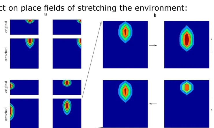
Effect on place fields of stretching the environment:
Manipulating the environment 2
Figure a: The place fields of four selected cells in the original and the stretched environment; the firing rates shown are averages over all head directions.
Figure b: Directionality of the place field shown in the bottom right corner of a; the place field depends on the heading of the rat (indicated by the arrows). This dependence on head direction is induced by the transformation of the environment; place fields in the original environment are essentially non-directional.
Idealized learning
Learning rule: associative - weight decay
Modulation: binary, global
Exploration model: Assume equal exposure to all possible locations and head directions in environment
Result:
Correctly models many properties of place fields, e.g. task-dependent
directionality
Exploration and exposure
Does the learning procedure actually work in real time?
Exposure:
Sample path:
An example trajectory, showing the first 5 minutes of exploration in a common paradigm in which the rat chases food pellets thrown into random locations in the
environment.
Sampling density as a function of position obtained by
convolving the sample path
with a Gaussian function.
Place cell firing after naive on-line associative learning:
Spatial representation
Place fields do not form correctly.
Learning continuous attractors
Uneven exploration results in substantial deviation from "ideal" weight structure:
•
random noise - mostly harmless
•
systematic bias - destroys attractor structure
Problem cannot be solved by using a modified learning rule involving
the same quantities.
Familiarity-gated learning
Try to equalize the amount of learning at different locations by modulating the learning rate:
Use exposure measure
to define novelty:
Choose optimally -> regular weight structure after 5 min
Naive on-line associative learning: Familiarity-gated learning:
Spatial representations
Place cell firing patterns during recall, after using different learning procedures.
The figure shows the firing rate maps of 18 randomly selected CA3 place cells after the exploration using simple Hebbian learning (left) and using the
familiarity-based learning procedure to establish the weights (right).
Further Results – very different environments
Figure: The place fields of five selected place cells in a rectangular and a circular apparatus that have very different sensory features.
The top row (R1) shows the place fields after learning in the rectangular apparatus but before any experience in the circular one, and the middle and
bottom rows show the place fields in the circular and rectangular environments (C and R2, respectively) after the rat has become familiar with both.
There is no obvious relationship between place fields of the same cell in the two environments. The effect of encoding a second environment on the place cell
representation in the first environment can be assessed by comparing the top and bottom rows. Although there are some visible changes, these tend to be small and do not affect the general structure of the spatial representation.
Overlapping attractors can also be encoded:
Experiment by Skaggs and McNaughton, 1998: Animals explored an apparatus that consisted of two visually identical boxes connected by a corridor. Many place cells were found to have similar place fields in the two regions, whereas others had uncorrelated place fields.
Further Results – very similar environments
Figure: The place fields of five CA3 place cells in the two identical boxes in the model; activity in the corridor connecting the boxes was not simulated.
The model has no difficulty storing and recalling partially overlapping spatial representations, because the degree of overlap is determined by what proportion of granule cells distinguishes between the two boxes in DG; CA3 cells simply inherit the selectivity of their MF inputs as attractors are established during the learning phase.
Overview
In this lesson we analyzed two models of short-term memory, and models of long-term memory. We learned about:
• The basic properties of short-term memory: can only store a few items at one time, requires persistent neural activity to maintain memory traces and can only store items for a limited amount of time.
• We analyzed a model by Brunel et al., which suggests that persistent activity is generated within a local cortical circuit, recurrent synaptic excitation is largely mediated by NMDA receptors, and recurrent network interactions are dominated by synaptic inhibition. With these assumptions the model is able to maintain persistent activity even in the presence of distractors, if the intensity of the distractor is not too high.
• Next we analyzed a model by Machens et al., who proposed a combined model of short- term memory and decision making. The model integrates short-term memory storage, maintenance, recall and comparison because its dynamical properties are easily controlled without changing its connectivity. The network exhibits mutual inhibition between nonlinear units, which makes it easily possible to construct networks with multiple behaviors.
• Finally we learned about a CA3 attractor network model by Káli et al. In this model local, recurrent, excitatory and inhibitory interactions generate appropriate place cell representations from location- and direction-specific activity in the entorhinal cortex.
Familiarity with the environment influences the efficacy and plasticity of the recurrent and feedforward inputs to CA3. Depending on the training experience provided, the model generates place fields that are either directional or nondirectional and which change in accordance with experimental data when the environment undergoes simple geometric transformations.