Development of Complex Curricula for Molecular Bionics and Infobionics Programs within a consortial*
framework**
Consortium leader
PETER PAZMANY CATHOLIC UNIVERSITY
Consortium members
SEMMELWEIS UNIVERSITY, DIALOG CAMPUS PUBLISHER
The Project has been realised with the support of the European Union and has been co-financed by the European Social Fund ***
**Molekuláris bionika és Infobionika Szakok tananyagának komplex fejlesztése konzorciumi keretben
***A projekt az Európai Unió támogatásával, az Európai Szociális Alap társfinanszírozásával valósul meg.
PETER PAZMANY CATHOLIC UNIVERSITY
SEMMELWEIS UNIVERSITY
Peter Pazmany Catholic University Faculty of Information Technology
MODELLING NEURONS AND NETWORKS
Lecture 3
Voltage-gated conductances
www.itk.ppke.hu
(Idegsejtek és neuronhálózatok modellezése)
(Feszültségfüggő ioncsatornák)
Szabolcs Káli
Overview
In this lesson you will learn first about voltage-dependent
conductances, and the importance of analyzing steady-state currents.
Next about the Hodgkin-Huxley model, which is the most widely used model for ion channels because of the good precision and flexibility to describe various currents. Then we will learn about the properties and models of synaptic channels.
Lesson topics:
• Voltage dependence of the membrane current
• Steady-state currents
• The Hodgkin-Huxley model, analysis of the model
• Characteristics of synaptic inputs
• The NMDA-type receptor
• Shunting synaptic inhibition
Voltage dependence of the membrane current
Special case:
In the most general case the membrane current is a function of the membrane potential and time:
The membrane current is a function of the membrane potential only (time-independent case).
We measure the total membrane current of a point neuron at different holding potentials.
Voltage dependence of the membrane current
We can define the chord conductance:
And the slope conductance:
More special case: , linear membrane, in this case both slope and chord conductance are equal to gm at any potential
In the general, time-dependent case
The instantaneous and steady-state current are usually measured.
The immediate and the steady-state (slope and chord) conductance can be defined too:
Upper plot: membrane current over time during voltage
clamp.
Instantaneous (dashed line) and steady-state currents in a neuron.
Instantaneous and steady-state current
Voltage-dependence of single ion currents
(reversal potential), and current always flows in the direction opposite to the electrochemical gradient, so the chord conductance
is always positive (the slope conductance can be either negative or positive).
The consequence is that passive ion currents can always be written as the product of the positive gi conductance and the Vm-Ei „driving
force”.
Every aforementioned definition is applicable to single ion currents.
In the case of passive membrane currents, it is known that if Ii=0
Voltage-dependent conductances
Single ion channels are either in an open or a closed state. The probability of the states can depend on the membrane potential and on the binding of various substances (e.g. neurotransmitters) to receptors in the cell membrane.
Figure: The currents passing through a single ion channel. In the open state, the channel passes -6.6pA at the holding potential of - 140mV. This is equivalent to more than 107 charges per second passing through the channel.
This means that for K+ ions to pass, 4 gates need to be open.
Example: In the case of the "delayed rectifier" K+ current:
Conductance per unit area of membrane for channel type i:
Where
Pi is the probability of a single channel being in the open state.
This is approximately equal to the fraction of open channels (if the number of channels is large).
is the maximal conductance per unit area of membrane.
Structurally, ion channel pores have numerous gates, which all need to be open for current to flow through the channel.
The Hodgkin-Huxley model
Gating equation
The transition of each gate is described by a kinetic scheme in which the gating transition closed-to-open occurs at voltage-dependent rate
and the reverse transition occurs at rate n is the probability that we find a gate open.
Left: example transition functions plotted as a function of the membrane potential
Gating equation (other form) The same equation in a useful form:
where
is called the time constant and
is the steady-state activation function.
Transient currents
Simplified description: activation and inactivation gate(s)
Example: transient Na+ current: The channel has k=3 activation and 1 inactivation gates:
activation – deactivation deinactivation - inactivation
Left: steady-state activation (n,m) and inactivation (h) curves plotted for the Na and delayed rectifier K channel. It describes the fraction of channel gates that will be open if the membrane potential is clamped to V for a long time. For example the m gate will be ~50% open at -40mV.
Right: time constant functions for the gates. This function describes how fast the channel gate will reach its steady-state activation.
Na and K channel example
Biophysical (kinetic) models of ion channels
HH-like Na+ channel:
Example: Hodgkin-Huxley-like K+ channel:
Smooth line: current predicted by the continuum model. Noisy curve:
simulation of individual channels.
Action potential
The full model of the giant squid axon with perfect „space clamp”:
The model includes:
-Na conductance with 3 activation gates and 1 inactivation gate, -K conductance with 4 activation gates.
-A passive leak conductance (the current flowing through the conductance is in linear relation with the membrane potential).
Squid axon HH model
Figure A: Currents flowing through the Na and K channels during an action potential.
Figure B: Membrane potential during an action potential.
Figure C: Activation and inactivation values during the spike.
Analysis of the squid axon model: 1-D approximation
Because the dynamics of the m gating variable are much faster than those of the h and n gates, the dynamics in steady-state are
approximately
I0(V) is the total current flowing through the channel. In this case we define the resting potential to be 0mV, and the activation and
inactivation variables are either fixed to their values at rest (h(0),n(0)) or instantaneously follow their steady-state values (m∞(V)).
Since the analysis does not take the time-dependence of the slower
gating variables into consideration, it is valid only for regions where the membrane potential changes rapidly.
Analysis of the squid axon model: 1-D approximation
Plot of the steady-state dynamics of the squid axon model.
Thick line(I0): sum of the currents.
Because m changes much faster than h or n for rapid inputs, we assumed that m adapts instantaneously to its new value if V changes. If I is negative, the membrane potential will increase, and if I is positive, it will
If the current is negative, the derivative of V is positive, thus it increases over time.
Absolute and relative refractory states
For a few milliseconds after an action potential, it is impossible to elicit another action potential. This time interval is called the absolute refractory period. For a more extended period, it is more difficult to elicit action potentials; this is called the relative refractory period.
Picture: Input current ratio as a function of the interspike interval.
I1: Threshold strength of the first current injection I2: Threshold strength of the second current injection
Response to sustained current injection
Response to different strengths
of sustained current injections. Top: Average membrane potential
Bottom: firing frequency as a
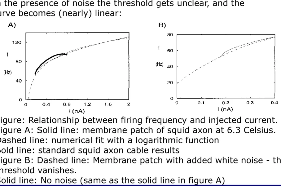
In the presence of noise the threshold gets unclear, and the curve becomes (nearly) linear:
Minimal spiking frequency
Figure: Relationship between firing frequency and injected current.
Figure A: Solid line: membrane patch of squid axon at 6.3 Celsius.
Dashed line: numerical fit with a logarithmic function Bold line: standard squid axon cable results
Figure B: Dashed line: Membrane patch with added white noise - the threshold vanishes.
Solid line: No noise (same as the solid line in figure A)
Propagation of the action potential
In this case
The general solution is not known, so we search for a wave-like solution, where V(x,t) = V(x-ut) (u is the propagation speed of the wave), and thus
Synaptic inputs
Synaptic activation causes a conductance change:
Isyn(t) = gsyn(t)(Vm(t) — Esyn)
Figure A: Excitatory postsynaptic current caused by activation of synapses (arrow)
Figure B: The peak postsynaptic current amplitude is in a linear relationship with the membrane potential.
Synaptic conductances
Where are synaptic transmitter concentration-dependent variables.
Assuming that the transmitter concentration changes as a square pulse, the synaptic current over time:
Phenomenological models of synaptic conductances
• Exponential (for example AMPA type glutamate receptor)
• Difference of exponentials (for example GABAA receptor). This
method uses two time constants, thus both rise and decay can be described
• Alpha function
This equation describes an isolated presynaptic release that occurs at t=0, reaches its maximum at the time constant, and decays with the time constant.
Figure: Example alpha function with Pmax=200 and tau=30.
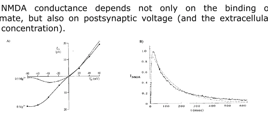
The NMDA-type glutamate synaptic receptor
Figure A: Current-voltage relations of the NMDA channel in the absence and in the presence of magnesium.
Figure B:
Jagged line: Experimentally recorded NMDA current.
Dotted line: computed NMDA current, with a double exponential time The NMDA conductance depends not only on the binding of glutamate, but also on postsynaptic voltage (and the extracellular Mg2+ concentration).
The NMDA-type glutamate synaptic receptor
To describe the Mg2+ dependence of the NMDA channel an additional factor is introduced, which depends on the postsynaptic potential:
Where P(t) is the open probability factor, and GNMDA(V) describes an extra voltage dependence due to the fact that near the resting potential NMDA receptors are blocked by Mg2+ ions, so to activate the conductance the postsynaptic neuron needs to be depolarized. This dependence can be approximated by a sigmoid function:
(typical fitted parameters: 1/η = 3.57 mM, 1/γ = 16.13 mV)
The NMDA channel also conducts Ca2+ ions, this is important in The NMDA-type glutamate synaptic receptor
Figure: Dependence of the NMDA conductance on the membrane potential at different Mg2+ concentrations.
Nonlinearity of synaptic input
Synaptic input to a passive compartment:
For slowly changing synaptic input:
Where
Synaptic inputs increase the membrane conductance and decrease the membrane time constant.
Nonlinearity of synaptic input
Steady-state membrane potential change due to synaptic input:
If there is a large EPSP, the cell membrane depolarizes, thus the synaptic driving force, Vm-Esyn decreases.
Figures: Synaptic input conductance characteristics. The effect of
varying the synaptic input conductance on the input conductance (A), the membrane time constant (B) and the steady-state membrane
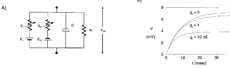
Shunting synaptic inhibition
Shunting inhibition is a type of inhibition where the reversal potential of the inhibitory synaptic channel is close to the resting potential of the cell.
As a consequence, the opening of the channel will introduce a current that changes the membrane potential towards the value of the resting potential.
For simplicity, we will use a single RC compartment:
Figure A: RC compartment used in the calculations. Ei=Vrest is the reversal potential of the synaptic channel.
Figure B: Depolarization of the membrane due to excitatory synaptic input combined with a shunting synaptic conductance of different strengths. The resting potential is 0mV. Increasing gi decreases the EPSP amplitude, and decreases the membrane time constant.
Shunting synaptic inhibition
The change in the membrane potential relative to the resting potential is:
This can be rewritten as (using the same notation as earlier):
Where the input conductance is:
And the time constant:
The steady-state membrane potential is:
Summary
In this lesson we learned:
• How the voltage-gated channels in cells function.
• How to describe them analytically: We use a formalism invented by Hodgkin and Huxley. In more detail:
• Instead of describing each channel individually, the conductance per unit area is measured. This is a power function, since each individual channel may
contain multiple gates, and current flows through the channel only if all the gates are open.
• The transitions of each gate are described by a kinetic scheme in which the gating transitions occur at voltage-dependent rates.
• With the help of the transition functions any voltage-gated channel can be described by its voltage-dependent time constant and steady-state activation functions.
• Next we constructed a squid axon model with active Na and K channels, and analyzed its behavior under different circumstances.
• Finally we modeled synaptic conductances, paying extra attention to the NMDA channel: The conductance of this channel depends not only on the binding of the transmitter, but also on the membrane potential.
Suggested reading Books:
•Christof Koch: Biophysics of computation, chapter 5
•Peter Dayan and L.F. Abbott: Theoretical Neuroscience, chapter 6
•Daniel Johnston, Samuel Miao-Sin Wu: Foundations of Cellular Neurophysiology
Articles:
•The original article about the Hodgkin-Huxley formalism: Hodgkin, A., and Huxley, A. (1952): A quantitative description of membrane current and its application to conduction and excitation in nerve. J. Physiol.
117:500–544.