Tools and Methods in Aiding Heat Exchanger Network Retrofit for Better
Economic Performance
PhD Thesis
Yong Jun Yow
Supervisor
Professor Dr. Jiří Jaromír Klemeš
Co-Supervisor Dr. Petar Varbanov
Doctoral School of Information Science and Technology University of Pannonia
Veszprém, Hungary 2018
DOI:10.18136/PE.2019.709
Tools and Methods in Aiding Heat Exchanger Network Retrofit for Better Economic Performance Thesis for obtaining a PhD degree in the Doctoral School of Information Science and Technology of the
University of Pannonia in the branch of Information Sciences
Written by Yong Jun Yow
Supervisor(s): Professor Dr. Jiří Jaromír Klemeš and Dr. Petar Varbanov
propose acceptance (yes / no) ……….
[SIGNATURE(S) OF SUPERVISOR(S)]
(supervisor/s)
The PhD-candidate has achieved ... % in the comprehensive exam,
Veszprém/Keszthely, [DATE] ……….
[SIGNATURE OF THE CHAIRMAN OF THE EXAMINATION COMMITTEE]
(Chairman of the Examination Committee) As reviewer, I propose acceptance of the thesis:
Name of Reviewer: …... …... yes / no
……….
[REVIWER’S SIGNATURE]
(reviewer) Name of Reviewer: …... …... yes / no
……….
[REVIWER’S SIGNATURE]
(reviewer) The PhD-candidate has achieved …...% at the public discussion.
Veszprém/Keszthely, [DATE] ……….
[SIGNATURE OF THE CHAIRMAN OF THE COMMITTEE]
(Chairman of the Committee) The grade of the PhD Diploma …... (…….. %)
Veszprém/Keszthely, [DATE]
……….
[SIGNATURE OF THE CHAIRMAN OF UDHC]
(Chairman of UDHC)
Acknowledgement
First and foremost, I would like to offer my highest gratitude to my supervisors, Professor Dr. Jiří Jaromír Klemeš and Dr. Petar Varbanov. I cannot possibly express anymore of my gratitude to them, not only on the guidance they gave during my study as a PhD student but valuable life experiences as well. Being in another county that is far away from home, they constantly make sure that my well-being was taken care off. Even when we are at different parts of the globe sometimes, they never give up on me and keep on guiding me so that I am on track. I would like to thank my family and Keat Liong for being there with me mentally, especially the three years when I was not in Malaysia. They support every decision I made without questioning. They reminds me of home when I am far away.
I would also like to take this opportunity to thank DDr. Lam Hon Loong and DDr. Andreja Nemet.
They provides ideas and tremendous help to me during my studies. There will never be enough of thank you and sorry from me for all the trouble I had caused them. I would like to thank the staff from University of Pannonia, especially Mrs Ujvári Orsolya and Mr Dulai Tibor. They assisted me in every possible way and went through all the office works for me to have a good experience in Hungary. I would like to thank my friends, Mr How Bing Shen, Mr Hong Boon Hooi, Mr Goh Wui Seng, Mr Lee Chit Seng and Miss Lim Li Sher. Lastly, I would like to thank all the collaborators and everyone who helped me during my journey as a PhD student.
Jun Yow YONG, 2018
Abstract
This thesis presents novel tools and methods developed specifically to be used during Heat Exchanger Network retrofit for better economic performance. The very first step in starting a retrofit process is collecting and extracting data from measured sets of process data. In the first discovery of this work, a novel method is proposed to ease the process of reconciling data of Heat Exchanger Network for the purpose of Heat Integration analysis. An iterative Method is introduced in the first part of this work differs from conventional data reconciliation method. The method is explained in detail - including its models used and algorithms. Two case studies, an illustrative and an industrial, successfully demonstrate the application of the method. Detailed discussions are given such as the effect of starting parameters to reconcile on the result. A limitation of the Iterative Method was identified and several strategies has been developed to overcome it. In the case studies, the strategies combining the Iterative Method are able to yield satisfying results. This comes at the expense of additional parameters into the models. The scope of data reconciliation is then expended to Total Site. Considering the complexity of Total Site, the model only includes utility systems and equipment, such as heaters, coolers and turbines. Heat exchangers in each individual plant are not considered in the model.
After obtaining the reconciled set of parameters, the next step is to represent them related to the Heat Exchanger Network structure. While the conventional Grid Diagram contains sufficient information for the retrofit process, it does not visualise the data sufficiently well for user interaction and decision making. The second discovery introduces a novel tool to represent all data required for Heat Exchanger Network retrofit in more detail, better supporting the engineer decision during the retrofit process. This tool is the Shifted Retrofit Thermodynamic Diagram. It includes the characteristics of Pinch Analysis. It can be used to easily identify not only the Process Pinch, but also any Network Pinch as well as Utility Pinch occurrences. With better visualisation, several ways are discussed of how to utilise this novel tool for better increase in heat recovery. A case study from the literature is used extensively to demonstrate the use and usefulness of Shifted Retrofit Thermodynamic Diagram.
Although a retrofit action can be thermodynamically feasible, it might not be economically feasible to be implemented. The last chapter is about the discovery of an alternative method to retrofit an existing Heat Exchanger Network, particularly reusing the waste heat. It is demonstrated using a real industrial case study, where it requires a large amount of investment cost to achieve the first retrofit result. In the case study, it is proposed otherwise that the waste heat is reused to heat up some streams. This reduces the utilities consumptions. Although it is similar to the initial proposed retrofit suggestion in terms of utilities saved, performs much better in terms of cost savings and payback.
Összefoglaló
Ez a doktori értekezés új eszközöket és módszereket mutat be, amelyek a specifikusan a hőcserélő hálózat módosítására lettek kifejlesztve. A módosítási (retrofit) folyamat legelső lépése az adatgyűjtés és kivonás a folyamat-adatok mért készleteiből. A munka első felfedezése egy új módszer javaslata, amely megkönnyíti az hőcserélő hálózatokra vonatkozó adatok összeegyeztetését a hő-integrálás elemzésére. Ezen munka elején bemutatott iteratív módszer különbözik a hagyományos összeegyeztetés módszertől. A módszert részletesen ismertetjük – beleértve a felhasznált modelleket és algoritmusokat. Bemutatjuk a részletes értekezést mint pl. az összeegyeztetés kezdő paramétereinek a hatása az eredményekre. Az iteratív módszer hátrányait azonosítottuk és különböző stratégiákat fejlesztettünk ki a hátrányok megoldására. Az esettanulmányokban az iteratív módszerek különböző stratégiáinak az egyesítésével elfogadható eredményeket értünk el. Ez a nagyobb számú paraméterek felhasználásával érhető el. Az adatok összeegyeztetését ezután kiterjesztettük az ún. Total Site szintre. A Total Site bonyolultságát figyelembe véve, a modell magába foglalja a segédközeg- rendszert és felszerelést, mint pl. a fűtők, hűtők és turbinák, viszont a hőcserélők az egyes üzemekben nem szerepelnek a modellben.
Az összeegyeztetett paraméter készletek elérése után, a következő lépés ezek bemutatása volt a hőcserélő hálózat struktúrájával összefüggésben. Míg a hagyományos rácsábrázolás elég információt tartalmaz a retrofit folyamathoz, nem tartalmaz elég adatot a felhasználó interakciójához és döntés hozatalához. A második felfedezés bevezet egy új eszközt a hőcserélő hálózat módosításához a szükséges részletes adatok bemutatására, amely jobban támogatja a mérnökök döntéseit a módosítás folyamatában. Ez az eszköz a módosított retrofit termodinamikai diagram (angolul: Shifted Retrofit Thermodynamic Diagram). Ez tartalmazza a pinch elemzés jellemzőit. Az eszközt fel lehet használni nem csak a folyamat pinch, hanem a hálózati pinch valamint a segédközeg pinch előfordulásának a meghatározására. A jobb vizualizálással, az új eszköz többféle felhasználását tárgyaljuk meg a hő-visszanyerés jobb növekedés érdekében. Irodalmi esettanulmány használtunk fel a módosított retrofit termodinamikai diagram felhasználásának és hasznosságának a bemutatására.
A termodinamikailag megvalósítható retrofit tevékenységek gazdaságilag nem feltétlenül megvalósíthatóak. Az utolsó fejezet a meglévő hőcserélő hálózat alternatív retrofit módszer felfedezést tárgyalja, különösen a hulladék-hő újrafelhasználásával. A módszer reális ipari esettanulmány felhasználásával kerül bemutatásra, amelynek magasak a beruházási költségei az első retrofit javaslatok elérésére. Az esettanulmányban a hulladék-hő újrafelhasználása javasolt némely áramok fűtésére. Ezzel csökkentjük a segédközegek felhasználását. Bár a javasolt megoldást hasonlít az eredeti javasolt módosításhoz a segédközegek felhasználásának a csökkentése szempontjából, sokkal jobban teljesít a költségek megtakarítás és a megtérülés szempontjából.
Table of Contents
Acknowledgement...i
Abstract...ii
Összefoglaló...iii
1. Introduction...1
1.1 References...3
2. Research Goals...6
3. Iterative Method for Data Reconciliation on Energy System...9
3.1 Introduction...9
3.2 Iterative Method for HEN in a Single Site...10
3.2.1 Problem Statement...10
3.2.2 Iterative method and models...12
3.2.3 Illustrative Case Study...13
3.2.4 Industrial Case Study...21
3.3 Limitation and Strategies for Application of the Iterative Method...24
3.3.1 Strategies Employed to Solve the Limitation...26
3.3.2 Illustrative Case Study – HEN Loops...27
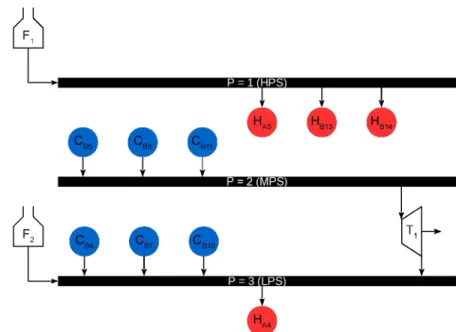
3.4 Data Reconciliation on Utility System of a Total Site...31
3.4.1 Problem Statement...31
3.4.2 Assumptions and Equations Used...32
3.4.3 Illustrative Case Study...38
3.4.4 Industrial Case Study...41
3.5 Summary...45
3.6 Nomaclatures...45
3.7 References...46
4. Advanced Visualisation for Retrofitting Heat Exchanger Network in Heat Integration... ... 47 4.1 Introduction...47
4.2 Shifted Retrofit Thermodynamic Diagram...48
4.2.1 Heat Path Development Considerations...53
4.2.2 Using SRTGD in Heat Path Development Steps for Identifying HEN Retrofit
Options ...58
4.2.3 SRTGD assessment...61
4.2.4 Case Study Implementing SRTD...62
4.2.5 Summary...73
4.2.6 Nomenclature...73
4.3 Heat Exchanger Matrix...74
4.3.1 Matrix Construction and Structure Description...74
4.3.2 Heat exchangers considered along a heat path...76
4.3.3 Case Study Implementing HEM...77
4.3.4 Summary...79
4.4 Conclusion...80
4.5 References...80
3. Heat Exchanger Network Modification for Waste Heat Utilisation...82
3.1 Introduction...82
3.2 Methodology...84
3.2.1 Parallel water heating with splitting the utility generation stream...84
3.2.2 Series heating of the utility generation stream...85
3.2.3 Combination of parallel and series heating...86
3.3 Case Study...87
3.3.1 Illustrative Case Study...87
3.3.2 Industrial Case Study...88
3.4 Summary...93
3.5 References...93
4. Novel Scientific Developments in the Current Thesis...94
5. Conclusions...95
Appendix...vi
Appendix 1...vi
Appendix 2...vii
1. Introduction
It has been four decades since Heat Integration analysis has been introduced for energy recovery in chemical plants (Klemeš and Kravanja, 2013). An important part of physical-insight methods is Process Integration. One of the first works on this has been that of Linnhoff and Flower (1978). The development up to present level has been summarised elsewhere (Klemeš et al., 2014) and specifically for Heat Integration in (Klemeš and Kravanja, 2013). Bakhtiari and Bedard (2013) modified the Network Pinch Approach to handle more complex networks with stream segmentation and splitting, also using heat exchanger specific values for the minimum allowed temperature difference.
Mathematical Optimisation usually employs algebraic models to solve the retrofit problem. Yee and Grossmann (1990) proposed a MINLP model with a stage-wise superstructure. Due to the numerical difficulty of solving the MINLP model, a number of options and assumptions are considered in a specialised superstructure. Bogataj and Kravanja (2012) proposed another alternative strategy for global optimization of HENs. The global optimal result is obtained on small HEN synthesis and good locally optimal solutions for larger problems. A recent mathematical model has been developed by Sreepathi and Rangaiah (2014) that uses continuously varying heat capacity. They apply single and multiple objective optimisation. As the next logical step from the retrofit of single process, the scope has been extended to cover Total Sites. For example, Liew et al. (2014) analysed all the streams involved in Total Site Heat Integration. They present a retrofit framework to determine the most cost-effective retrofit options and maximise the potential savings.
While it is important to have Heat Integration in chemical plants, retrofitting an existing HEN is also important (Klemeš, 2013). It is observed that the recent focus of Heat Integration has shifted towards retrofitting existing chemical plants. This is due to existing Heat Exchanger Networks (HEN) have become obsolete after years of service. Chemical, petrochemical, power and other industries are keen to improve the energy efficiency of their plants due to the energy cost (BP, 2013) and increasingly strict environmental regulations (European Commission, 2011).
With current fluctuating energy prices, increased production and change in process equipment, retrofitting can reduce operating cost with some capital investment. Various methods have been published for solving the retrofit problem. They are generally based on physical insight, mathematical optimisation or combination of both.
During the HEN retrofit process, most of the attention is given to how the network can achieve better heat recovery or throughput. The steps on how to collect and process data from HEN to be used in the analysis are usually given very little attention. From the search in the literature, very few research works are available on heat exchanger data acquisition and processing, let alone on HEN. One of the early works, that could be found, is by Shenoy (1995). In that, the data reconciliation problem is modelled by Nonlinear Programming, based on average measurement values. The model formed the very base tool set that is even used until today.
From there, ways of solving the model to obtain the reconciled result are developed.
The model can be solved as it is with the current computer technology and advancement. As shown in part of the current thesis by Yong et al. (2016), the data reconciliation model is solved simultaneously (i.e. solving for all unknowns at the same time). It was performed using a Local solver GAMS/CONOPT with the global optimization algorithm (GOA) reported in Faria and Bagajewicz (2011). The original non-convex nonlinear optimisation problem was converted into a convex one by replacing the bilinear terms with McCormick’s envelopes. It might be deemed too difficult for user without advanced mathematical and computational knowledge.
The book by Narasimhan and Jordache (2000) covers provides basic introduction, explanations and ways to solve the data reconciliation problems. Among the methods mention in the book, one of the simpler method to solve the problem is Modified Iterative Measurement Test (MIMT).
Details of the method are not discussed here. The method employs the use of matrix and equations involving statistical calculation to find the result. It is possible to be solved manually or implemented into Microsoft Excel. For example, detailed usage and discussion of this method can be found in the master’s thesis work of Mayo (2015). It should be noted that the method is only capable of solving one type of parameter. For the case of data reconciliation for the purpose of Heat Integration analysis, which contains two types of parameters, the method is deemed unsuitable. For this reason, a non-simultaneous data reconciliation algorithm on HEN was introduced in the work of Ijaz et al. (2013). It involves using formulae to reconcile one parameter via QR factorisation. The idea of the non-simultaneous method is good but is also not suitable for the purpose of Heat Integration analysis as it includes the overall heat transfer coefficient for each heat exchanger, which is irrelevant to some types of Heat Integration analysis.
The Grid Diagram is the most common way of representing a HEN during Heat Integration analysis. Particularly for an insight-based method such as Pinch Analysis, after targeting minimum utility consumption, the HEN design is done on the Grid Diagram. Streams are represented as horizontal lines with individual heat capacity flowrates. The direction of the line depends on the nature of the streams with the starting and ending temperatures indicated at the ends of the line. With identified Pinch temperature, the HEN is designed according a set of algorithms by connecting the horizontal lines with vertical lines representing heat exchangers.
The designed HEN will finally achieve the targeted result. As for designing a HEN using mathematical optimisation, the whole process does not require the visualisation of HEN. It is however that the final result will represented on HEN grid diagram. Beside Grid Diagram, there are other visualisation tools to represent HEN. For example, Retrofit Thermodynamic Diagram (RTD) by Lakshmanan and Bañares-Alcántara (1996), Heat Loads Plot by Piacentino (2011) and Streams Temperature vs. Enthalpy Plot (STEP) by Wan Alwi and Manan (2010). Gadalla (2015) plotted temperatures of hot process streams versus cold process streams. Further discussions of these tools are made in Section 4.1. While these tools are used to design HEN, the usability on HEN retrofit process is not made known by the authors.
Most of HEN retrofit procedures are performed using mathematical optimisation. Due to the mathematical optimisation, it is possible to include more objectives in the model during the
retrofit process. To list a few, in the work of Kang and Liu (2017), a systematic strategy for multi- period HEN is developed with the objective of minimising the total annual cost and total annual carbon dioxide emissions. Ayotte-Sauvé et al. (2017) uses superstructure with new stepwise approach to optimise the HEN retrofit. Using new algorithms and at each iteration, these superstructures are thinned out to reduce calculation times. Other consideration can also be included during the retrofit process, as shown in the work of Rangfak and Siemanond (2017).
The proposed model is based on stage-wise superstructure with fouling effect included. Using a crude oil preheat train as case study, the large-scale MINLP problem is solved by applying initialisation and sequential techniques.
There are HEN retrofit procedures based on insight. Tjoe and Linnhoff (1986) are some of the first to use Pinch Technology for HEN retrofit. Following on that, Li and Chang (2010) have eliminated cross-Pinch heat transfer in HENs using Pinch Analysis. In the work of Smith and Akpomiemie (2017), heat transfer enhancement is focused to reduce the number of structural modification and minimize the capital investment. The work presents a new Pinch retrofit method for structural modifications and a combined method that simultaneously considers enhancement alongside structural modification. Bonhivers et al. (2017) claimed that mathematical approaches to HEN retrofit are complex and do not guarantee the global optimum. In the first part of the work, an energy transfer diagram called Energy Transfer Diagram (ETD) is proposed. The graphical approach to identify the heat exchanger configurations is shown to be able to reduce the energy consumption. The authors claimed that the method is practical, visual and user-friendly.
For HEN retrofit an interesting concept has been introduced by Asante and Zhu (1996). Their discovery of the Network Pinch (NP) that occurs due to HEN topology has provided key insights into the HEN retrofit problem. The location of the NP is determined by the HEN topology limitations, so it is usually different from the Process Pinch (PP) Temperature identified using Pinch Analysis. The NP concept has proved beneficial in retrofitting existing HENs.
1.1 References
Asante, N.D.K., Zhu X.X., 1997, An automated and interactive approach for heat exchanger network retrofit, Chemical Engineering Research and Design, 75(part A), 349-360.
Ayotte-Sauvé E., Ashrafi O., Bédard S., Rohani N., 2017, Optimal retrofit of heat exchanger networks: A stepwise approach, Computers & Chemical Engineering, 106, 243-268.
Bakhtiari B., Bedard S., 2013, Retrofitting Heat Exchanger Network using a Modified Network Pinch Approach, Applied Thermal Engineering, 51 (1-2), 973 – 979.
Bogataj M., Kravanja Z., 2012. An alternative strategy for global optimization of heat exchanger network, Applied Thermal Engineering, 43, 75 – 90.
Bonhivers J.-C., Alva-Argaez A., Srinivasan B., Stuart P.R., 2017, New analysis method to reduce the industrial energy requirements by heat-exchanger network retrofit: Part 2 – Stepwise and graphical approach, Applied Thermal Engineering, 119, 670-686.
BP, 2013, BP Statistical Review of World Energy June 2013, <www.bp.com/content/dam/bp/
pdf/statistical-review/statistical_review_of_world_energy_2013.pdf> accessed 01.04.2014 European Commission, 2011, Poor Energy Use is Chemical Industry’s Top Environmental Issue,
Science for Environment Policy, <ec.europa.eu/environment/integration/research/
newsalert/pdf/243na2_en.pdf> accessed 09.01.2014
Faria D.C., Bagajewicz M.J., 2011, Novel bound contraction for global optimization of bilinear MINLP problems with applications to water management problems, Computers and Chemical Engineering, 35, 446–455.
Gadalla M.A., 2015, A new graphical method for Pinch Analysis applications: Heat exchanger network retrofit and energy integration, Energy, 81, 159 – 174.
Ijaz H., Ati U. M. K., Mahalec V., 2013, Heat exchanger network simulation, data reconciliation &
optimization, Applied Thermal Engineering, 52(2), 328 - 335.
Kang L., Liu Y., 2017, A systematic strategy for multi-period heat exchanger network retrofit under multiple practical restrictions, Chinese Journal of Chemical Engineering, 25(8), 1043- 1051.
Klemeš J.J. Kravanja Z., 2013. Forty years of Heat Integration: Pinch Analysis (PA) and Mathematical Programming (MP), Current Opinion in Chemical Engineering, 2(4), 461 – 474.
Klemeš J.J., 2013, Handbook of Process Integration (PI): Minimisation of Energy and Water Use, Waste and Emission, Woodhead Publishing/Elsevier: Cambridge, UK
Klemeš J.J., Varbanov P.S., Wan Alwi S.R., Manan Z.A., 2014, Process Integration and Intensification: Saving Energy, Water and Resources, Walter de Gruyter: Berlin, Germany Lakshmanan R., Bañares-Alcántara R., 1996, A Novel Visualisation Tool for Heat Exchanger
Network Retrofit, Industrial & Engineering Chemistry Research, 35, 4507-4522.
Li B.-H., Chang C.-T., 2010. Retrofitting heat exchanger networks based on simple pinch analysis, Industrial & Engineering Chemistry Research, 49(8), 3967 – 3971.
Liew P.Y., Lim J.S., Wan Alwi S.R., Manan Z.A., Varbanov P.S., Klemeš J.J., 2014, A retrofit framework for Total Site heat recovery systems, Applied Energy, 135, 778 – 790.
Linnhoff B., Flower J.R., 1978. Synthesis of heat exchanger network: I. Systematic generation of energy optimal networks, AlChE Journal, 24, 633 – 642.
Mayo C.M., 2015, Process Stream Data Analysis: Data Reconciliation and Gross Error Detection for Process Integration Studies, Master’s Thesis, Chalmers University of Technology.
Narasimhan S., Jordache C., 2000, Data Reconciliation & Gross Error Detection: An Intelligent Use of Process Data, Gulf Publishing Company, Houstan, Texas.
Piacentino A., 2011, Thermal Analysis and New Insights to Support Decision Making in Retrofit and Relaxation of Heat Exchanger Networks, Applied Thermal Engineering, 31(16), 3479 – 3499.
Rangfak S., Siemanond K., 2017, Heat Exchanger Network Retrofit with Fouling Effects, Computer Aided Chemical Engineering, 40, 775-780.
Shenoy U.V., 1995, Heat exchanger network synthesis, Gulf Professional Publishing, Houston, USA.
Smith R., Akepomiemie M.O., 2017, Low Cost Retrofit Methods for Heat Exchanger Networks, Computer Aided Chemical Engineering, 40, 1789-1794.
Sreepathi B.K., Rangaiah G.P., 20154, Retrofitting of Heat Exchanger Networks Involving Streams with Variable Heat Capacity: Application of Single and Multi-Objective Optimisation, Applied Thermal Engineering, 75, 677 – 684.
Tjoe T.N., Linnhoff B., 1986. Using Pinch Technology for process retrofit, Chemical Engineering (New York), 93(8), 47 – 60.
Wan Alwi S.R., Manan Z.A., 2010, STEP – A new graphical tool for simultaneous targeting and design of a heat exchanger network, Chemical Engineering Journal, 162(1), 106 – 121.
Yee T.F., Grossman I.E., 1990, Simultaneous optimization models for heat integration – II. Heat exchanger network synthesis, Computers & Chemical Engineering. 14(10), 1165 – 1184.
Yong J.Y., Nemet A., Bogataj M., Zore Ž., Varbanov P.S., Kravanja Z., Klemeš J.J., 2016, Data Reconciliation for Energy System Flowsheets, Computer Aided Chemical Engineering, 38, 2277-2282.
2. Research Goals
The general process of retrofitting an existing heat exchanger network (HEN) for better heat integration can be divided into several stages. The first stage is to acquire data from the chemical plant. For this purpose, process flow diagram is used to have an overall view of the process and equipment of the plant. It is important that the boundary for heat integration analysis is defined, especially if it involves several plants together. The second stage of the process is data extraction. As the purpose is for heat integration analysis, only streams with changed temperature should be considered in the extraction. This is to avoid unnecessary data being extracted without being used. These streams can be easily identified as they pass through either heat exchanger, cooler or heater. Low grade heat such as in waste heat streams ejected to environment are also to be extracted.
After the relevant streams are being identified, repeated measurements of temperature and mass flowrate taken for a period of time of each stream are extracted. The repeated measurements are then processed to remove any outliers. For more details on data processing prior to data reconciliation, it is provided in the appendix section of this work. The topology of the HEN is also extracted. Data reconciliation is performed on the measurements in order to obtain a representative data that satisfy the system constraints. The third stage is heat integration analysis where retrofit options are explored and proposed. At this stage, the retrofit options are continuously send to industrial partner for feedback. If the retrofit option is found to be expensive in terms of investment or time, other options are explored such as generating side-product for extra revenue. Once the retrofit option is decided and finalised, implementation is performed on the chemical plant. The changes and results are recorded for future reference.
Data reconciliation has a wide implementation in the industry. On the search of the keyword
“Data Reconciliation” in scientific journal website, ScienceDirect shows more than thousands of work discussing data reconciliation on various processes and equipment. The current state of the art for data reconciliation is to employ an MINLP model to solve the data reconciliation problem. The model generally consists of an objective function that uses least square method and set of constraints governing the process or equipment. It is important to state the focus and purpose of the data reconciliation before it begins. As the main topic of this work is HEN retrofit, the focus is therefore on the HEN and the purpose is heat integration analysis. Narrowing down the search on data reconciliation on HEN, however to the knowledge of author, does not produce much finding in the literature. Although these works focus on HEN, the purpose for heat integration analysis is even fewer. For example, in the master’s thesis of Mayo (2015), Microsoft Excel is introduced to be used to perform data reconciliation due to its user friendly feature. In the work, it is also assumed that temperatures are the only adjustable variable, while the mass flowrates are kept constant. For heat integration analysis, both of these parameters are equally important and should not be left out in the data reconciliation process. The other works found are discussed in detail in chapter 3 in this thesis. Furthermore, on further investigation, certain
constraints used for data reconciliation poses additional complexity to the model. Of all the constraints used, energy balance constraint causes the non-linearity in the model.
The first main research goal is to develop a less computational effort requiring method during data reconciliation process with two types of parameters. The goal is then further extended to only include energy systems in data reconciliation process in Total Site. A new method is introduced to solve this non-linearity in section 3.2 that iterates between two linear sub-models.
Through case studies iterative method is shown to be able to provide satisfying result with less computational time. In section 3.3, limitation encountered when using iterative method is discussed. To overcome this limitation, three different strategies are developed. Section 3.4 presents a new way to solve data reconciliation problem on Total Site. Model to solve data reconciliation on utility system is presented with demonstration from both illustrative case study and industrial case study.
The topology data of HEN is crucial to heat integration analysis. While stream data can be stored in the form of table, the topology data of HEN cannot be stored easily in table form.
Although process flow diagram is able to show the whole HEN, it contains other equipment that is not relevant to heat integration analysis. The most conventional way of representing HEN is by using Grid Diagram. In the diagram, streams are involved in heat exchange is represented in horizontal lines. Heat exchangers are then shown in Grid Diagram connecting hot streams and cold streams vertically. Grid Diagram is used intensively in designing HEN especially after performing Pinch Analysis. Coupling with heuristic from Pinch Analysis, the found pinch divide HEN Grid Diagram into two parts where no heat transfer is allowed across the pinch. It should be noted that while Grid Diagram provides visualisation of the HEN, it is still lacking visual information of some other important parameters. Various studies are found in the literature to have added extra feature to improve the conventional Grid Diagram. For example, in the work of Gadalla (2015), HEN is represented in graph with cold process stream temperature in the x-axis and hot process stream temperature in the y-axis. From the graph it can be seen that improvement is made on visualising heat exchanger using arrow. The coordinates at the start and end of the arrow indicates the temperatures of both hot and cold streams. For other works it is discussed in chapter 4. However, according to the knowledge of author, there is still a need for a HEN representation that includes other important parameters to be considered during HEN retrofitting analysis. This includes location of pinches and mass capacity flowrates.
The second research goal is to develop HEN representations from conventional Grid Diagram to include more parameters for better visualisation and decision making. Referring to the second part of these research works, section 4 introduced an extended Grid Diagram – the Shifted Retrofit Thermodynamic Grid Diagram (SRTGD). SRTGD has unique feature set, helping to identify favourable retrofit options. It shows heat capacity flowrates (CP), temperatures and the network in the same view. It allows the users to simultaneously account for the thermodynamics, stream capacities and the topology as factors during heat recovery. The goal is further extended to develop a representation in the form of table without drawings. Later in the section the
suggestion to represent HEN numerically in a matrix form is proposed. HEN Stream Matrix (HENSM) is able to improve the discussed limitations faced by graphical representations.
While retrofitting HEN, the boundary is conventionally set only within the plant itself. Doing so may result in economically unfavourable option and missing other opportunity to utilise low grade heat. When retrofit for utilities usage reduction is deemed economically unfavourable for a HEN, the next level in hierarchy is to analyse heat utilisation options to produce value-added products. The last research goal is to identify other retrofit solutions when a thermodynamic driven retrofit solution is deemed economically infeasible. This is shown in the last part of these research works in section 5.
3. Iterative Method for Data Reconciliation on Energy System
3.1 Introduction
Data extraction is the very first and crucial step performed before any Heat Integration study can commence (Klemeš, 2013). Particularly for existing plants for retrofitting, data reconciliation is a step that must be performed in data extraction to obtain representative data (Klemeš and Varbanov, 2010). It is a procedure that extracts an accurate and reliable set of data from repeated raw measurements that satisfies the system constraints. Shenoy (1995) published a nonlinear programming model for Heat Exchanger Network (HEN) data reconciliation, based on average measurement values. Vocciante et al. (2014) developed a reconciliation strategy that assesses the convenience of using enthalpy balances in the reconciliation of flowrates. The resulting algorithm based on interval analysis provides a general framework on selection of equation to be used in reconciliation process. In the work of Kongchuay and Siemanond (2014), gross detection error technique is in data reconciliation to improve the data measurement of a simulated hot-oil heat exchanger using non-linear programming.
The main Heat Integration analysis method – Pinch Analysis, requires heat capacity flowrates (CP) and temperatures (T) of process streams. While there are already some publications on reconciliation of measured HEN data (Nemet et al., 2015), works presenting data reconciliation for Pinch Analysis are scarce. The models proposed in the literature reconcile CP and T simultaneously. A non-simultaneous data reconciliation algorithm on HEN was introduced in the work of Ijaz et al. (2013). It involves using formulae to reconcile one parameter via QR factorisation. Although the algorithm is non-simultaneous, it is non-iterative as well. It reconciles one parameter at a time and stops after reconciling the last parameter. The algorithm first reconciles mass flowrates using only mass balance equations and then proceeds to reconciling measured temperatures using energy balance equations where the already calculated mass flowrate values are supplied as fixed parameters. As only mass balance equations are used in the first step of the algorithm, the mass flowrate values have influence on the result when temperatures are reconciled. It is noted that the temperature values have no influence on the result when mass flowrates are reconciled.
There is a need for a method to solve data reconciliation suited to Heat Integration for retrofit.
The method should be easily understandable to the users who wish to perform data reconciliation without much knowledge in solving complex models and should require less computational effort. The method described in this work is only consists of linear constraints equations and linear least square method is used on objective function. User is then only required to have skills and knowledge in linear programming and coding using mathematical optimisation software. This chapter is composed of 3 main sections. First, in section 3.2, the new method, called iterative method is introduced. It allows overcoming the non-linear complexity in the data reconciliation model. Section 3.3 discusses the limitation encountered when using iterative method. A few strategies are developed to overcome this limitation. The last section being section 3.4 explores the use of iterative method on utility system found in Total Site Heat Integration.
3.2 Iterative Method for HEN in a Single Site
In data reconciliation on HEN, the only two types of parameters to be reconciled are heat capacity flowrates (CP) and temperatures (T) of process streams.
3.2.1 Problem Statement
Consider a single HEN, where it has heat exchangers and utility consuming equipment, i.e.
heaters and coolers. All this equipment are considered for data reconciliation. All heaters and coolers are modelled in exactly the same way as heat exchangers. It is because the only difference between these utility consuming equipment and heat exchanger is one of the streams is containing utility. These utility carrying streams can also be modelled as normal stream in the network. All equipment is labelled as i I. On every heat exchanger, there are two inlets (I) and∈ two outlets (O) for hot (H) and cold (C) streams. These generate a set of streams, s {HI, HO,∈ CI, CO}. Two types of parameters are only considered in the data reconciliation, which are temperature (T) and heat capacity flowrate (CP). Given a repeated set of measurements of all heat exchangers in a set period of time for n times, the aim is to find the corresponding reconciled parameters, RTi,s and RCPi,s for all heat exchangers.
Figure 3.1: Example of a HEN
Simultaneous Solving Method
Min
∑
i
I
∑
s
S
∑
n
N
( (
RCPi , s−CPi , s ,n)
2+(
RTi ,s−Ti ,s , n)
2)
(3.1)subject to:
Mass balance constraints around each heat exchanger, for all heat exchanger For example, HEX1 in Figure 3.1
RCP1,HI=RCP1,HO (3.2)
RCP1,CI=RCP1,CO (3.3)
Energy balance constraints around each heat exchanger, for all heat exchanger For example, HEX1 in Figure 3.1
RCP1,HI
(
RT1,HI−RT1,HO)
=RCP1,CI(
RT1,CO−RT1,CI)
(3.4)Constraints from network arising from the connections between heat exchangers For example, according to Figure 3.1
RCP1,HO=RCP2,HI (3.5)
RCP1,CO=RCP3,CI (3.6)
RT1,HO=RT2,HI (3.7)
RT1,CO=RT3,CI (3.8)
Figure 3.2: Data reconciliation model for solving two parameters simultaneously
Figure 3.2 shows the model is conventionally solved when two types of parameters are reconciled simultaneously. In this context this is a simultaneous method. Linear least square method Eq(3.1) is used in the objective function to find reconciled values of all parameters using statistically given data. Least absolute method can be used in objective function and doing so eliminates the non-linearity in the objective function. It is however that least square method provides better accuracy as larger sums are penalised more. Least absolute method also may cause discontinuous function in the model that needs extra coding. It should be noted that heat capacity, CP is expressed in Eq(3.9):
CP=cp×m´ (3.9)
where cp is the specific heat capacity of the stream and ṁ is the mass flowrate. cp is a function of T. Depending on the cp function found in literature, it has at least power of three of T.
Including this non-linear function into the model will cause it to be complex. Solving such highly non-linear model requires very high computational effort and time. The high non-linearity of the model also means no guarantees of finding the global optimum or – in extreme cases- even for numerical convergence. To reduce the degree of non-linearity, it is assumed that in this work cp is independent of T. Another factor which will increase the complexity of the model is the number of heat exchangers, which in turn affect the number of parameters to be reconciled.
There are three types of constraint equations used in the model. Mass balance constraint equations around a heat exchanger for all heat exchanger are shown in Eq(3.2) and Eq(3.3).
The equations are straight forward since the equations only involve RCP. There are also constraint equations from network, shown in Eq(3.5) and Eq(3.6). These equations are used when the outlet of a heat exchanger is connected to an inlet of another heat exchanger. Energy balance constraint equations are however complicating the model as shown in Eq(3.4) when solved simultaneously. This is due to the equations containing the product of RCP and RT. The products of these two parameters, if solved simultaneously, increase the difficulty to solve the model. Doing so requires more computational effort and time. To reduce the degree of non- linearity in the model, iterative method is introduced in this work.
3.2.2 Iterative method and models
The iterative method is an alternative to the simultaneous method. The method partitions the model used in the simultaneous method into two sub-models. Iterating between the two sub- models, the method keeps one type of parameters constant (e.g. T) while reconciling the parameters of the other type (e.g. CP), until satisfactory convergence is achieved. Two types of parameters are reconciled separately while still maintaining the importance of other parameters in the models. Although the iterative method features some inaccuracy, compared to the simultaneous method, it is significantly less computationally intensive and simple to implement.
Figure 3.3 shows the models used in iterative method. Compared to model shown in Figure 2.1, the constraint equations used are same except for the objective functions. Two models are used iteratively namely CP model and T model. CP model has only CP to be reconciled as shown in Eq(3.9) while keeping RT constant in Eq(3.4) and without Eq(3.7) and Eq(3.8). It is vice versa for T model. Each model shown is only required to reconcile one type of parameters. For CP model, it has both mass balance constraint and energy balance constraint equations. In the respective objective function in the models, the dimension of the parameters is the same, as this is not the case with simultaneous method.
CP Model T Model
Min
∑
i I
∑
s S∑
n N(
RCPi ,s−CPi , s ,n)
2 (3.9) Min∑
i I
∑
s S∑
n N(
RTi ,s−Ti , s ,n)
2 (3.10)subject to: subject to:
Mass balance constraints
RCPi , HI=RCPi , HO (3.2)
RCPi ,CI=RCPi ,CO (3.3)
Energy balance constraints Energy balance constraints
RCPi , HI
(
RTi , HI−RTi , HO)
=RCPi ,CI(
RTi ,CO(3.4)−RTi ,CI)
RCPi , HI(
RTi , HI−RTi , HO)
=RCPi ,CI(
RTi ,CO(3.4)−RTi ,CI)
where RT is set to be constant where RCP is set to be constant Constraints from network for example Constraints from network for example
RCPi1,HO=RCPi2,HI (3.5) RTi1,HO=RTi2,HI (3.7)
RCPi1,CO=RCPi2,CI (3.6) RTi1,CO=RTi2,CI (3.8) Figure 3.3: Equations used in CP model and T model
Figure 3.5 shows the algorithm to deploy these models. The algorithm starts with step 1 being collecting the necessary information for the data reconciliation problem. Step 2 is finding out the mean values of all parameters, which is important and will be used as the initial guess in either model. As for step 3, user has to choose either to reconcile CP or T first. For example, if CP is to be chosen to be reconciled first, the algorithm leads to step 3(a). Using the mean value of T found in step 2, substitute it into RT and solve using CP model to obtain RCP. Step 4(a) ensures that only one type of parameter is reconciled at a time. To obtain values for RT, the found value of RCP in step 4(a) is kept constant and substitute into T model in step 5(a). To find if the results are acceptable and consistence, in step 6, the percentage difference of the constant parameter in previous 2 steps and obtained parameter in previous step is calculated. That is, until this step, the percentage difference is calculated between constant RT values used in step 4(a) and reconciled RT values in step 5(a). If the percentage difference falls below satisfactory level, then proceed to and end at step 7. Else if it is not, then it should be iterated until it achieves the set satisfactory level. It should be noted that before step 6, reconciled RT values obtained in step 5(a) can be used in step 5(b). Then at step 6, the percentage difference is calculated between constant RCP values used in step 5(a) and reconciled RCP values in step 5(b). It is vice versa if T is to be reconciled first. The number of iterations is determined by the number of step 6 encountered. Overall if it does not stop at first iteration, the steps when choosing CP to be reconciled first would be:
1 → 2 → 3(a) → 4(a) → 5(a) → 6 → 5(b) → 6 → 5(a) → 6 → 5(b) →…→ 7 3.2.3 Illustrative Case Study
An illustrative case study is used to demonstrate the use of the algorithms. The HEN is shown in Figure 3.4. Over the years, the chemical plants underwent several modifications and twitching.
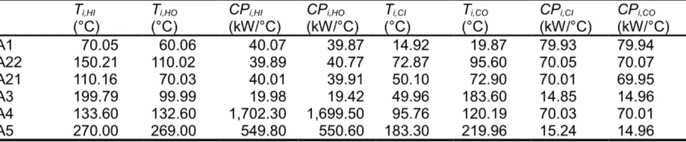
This resulted in changes in the heat exchangers as well. It is desired to retrofit the current HEN to achieve minimal utility consumption with limited investment cost. It is included in the data reconciliation problem. It is assumed that measurements are taken at every inlets and outlets of every heat exchangers, heaters and coolers. After sets of measurements are taken repeatedly for a fixed period of time, the outliers are discarded using statistics. Out of these sets of measurements, 10 are chosen to be used as the input data.
Figure 3.4: HEN for illustrative case study
Figure 3.5: Algorithms of proposed iterative method
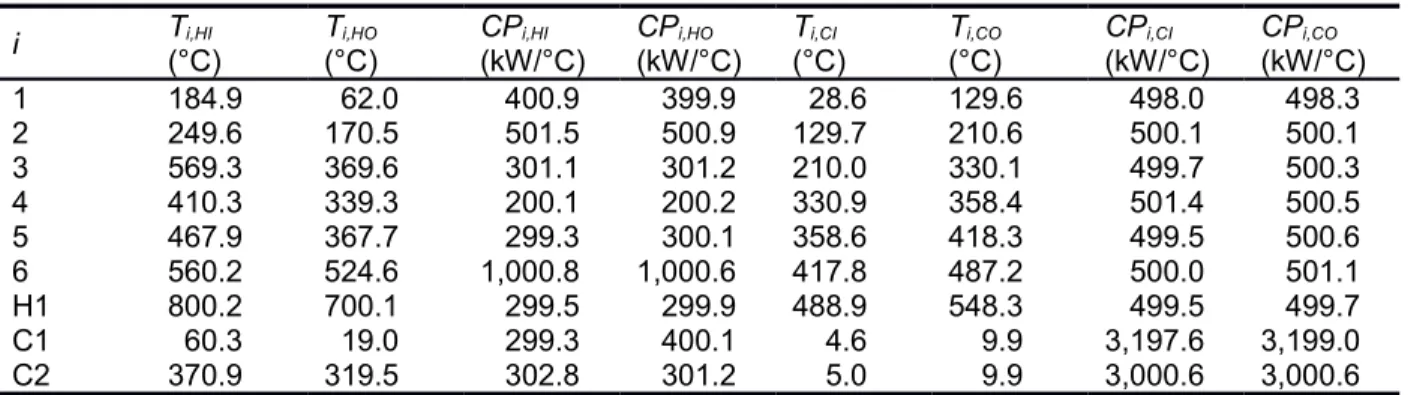
The next step is to calculate the mean values for all parameters. It is shown in Table 3.1.
Table 3.1: Mean values for all the parameters in the illustrative case study.
i Ti,HI
(°C) Ti,HO
(°C) CPi,HI
(kW/°C) CPi,HO
(kW/°C) Ti,CI
(°C) Ti,CO
(°C) CPi,CI
(kW/°C) CPi,CO
(kW/°C)
1 184.9 62.0 400.9 399.9 28.6 129.6 498.0 498.3
2 249.6 170.5 501.5 500.9 129.7 210.6 500.1 500.1
3 569.3 369.6 301.1 301.2 210.0 330.1 499.7 500.3
4 410.3 339.3 200.1 200.2 330.9 358.4 501.4 500.5
5 467.9 367.7 299.3 300.1 358.6 418.3 499.5 500.6
6 560.2 524.6 1,000.8 1,000.6 417.8 487.2 500.0 501.1
H1 800.2 700.1 299.5 299.9 488.9 548.3 499.5 499.7
C1 60.3 19.0 299.3 400.1 4.6 9.9 3,197.6 3,199.0 C2 370.9 319.5 302.8 301.2 5.0 9.9 3,000.6 3,000.6 Every heat exchanger has its own individual mass and energy constraint equations, for example for HEX-01:
RCP1,HI=RCP1,HO (3.11)
RCP1,CI=RCP1,CO (3.12)
RCP1,HI
(
RT1,HI−RT1,HO)
=RCP1,CI(
RT1,CO−RT1,CI)
(3.13)As for the constraints raised from network
RCP1,HO=RCPC1,HI (3.14) RT1,HO=RTC1,HI (3.22)
RCP3,HO=RCPC2,HI (3.15) RT3,HO=RTC2,HI (3.23)
RCP1,CO=RCP2,CI (3.16) RT1,CO=RT2,CI (3.24)
RCP2,CO=RCP3,CI (3.17) RT2,CO=RT3,CI (3.25)
RCP3,CO=RCP4,CI (3.18) RT3,CO=RT4,CI (3.26)
RCP4,CO=RCP5,CI (3.19) RT4,CO=RT5,CI (3.27)
RCP5,CO=RCP6,CI (3.20) RT5,CO=RT6,CI (3.28)
RCP6,CO=RCPH1,CI (3.21) RT6,CO=RTH1,CI (3.29)
In this case study, both CP and T solution routes will be investigated. In the following section has CP path is to be chosen first. It is decided that step 3(a) and 4(a) are to be followed next.
The mean value of T parameters are substituted and kept constant while solving the CP model.
The result after Step 4(a) is shown in Table 3.2.
Using the result in Table 3.2, in Step 5(a), RCP obtained is kept constant and RT is solved in T model. The result is shown in Table 3.3.
Table 3.2: Result for the illustrative case study after Step 4(a) in first iteration following CP path i Ti,HI
(°C) Ti,HO
(°C) CPi,HI
(kW/°C) CPi,HO
(kW/°C) Ti,CI
(°C) Ti,CO
(°C) CPi,CI
(kW/°C) CPi,CO
(kW/°C)
1 184.9 62.0 402.6 402.6 28.6 129.6 490.0 490.0
2 249.6 170.5 501.1 501.1 129.7 210.6 490.0 490.0
3 569.3 369.6 294.7 294.7 210.0 330.1 490.0 490.0
4 410.3 339.3 189.8 189.8 330.9 358.4 490.0 490.0
5 467.9 367.7 291.9 291.9 358.6 418.3 490.0 490.0
6 560.2 524.6 955.1 955.1 417.8 487.2 490.0 490.0
H1 800.2 700.1 290.7 290.7 488.9 548.3 490.0 490.0
C1 60.3 19.0 402.6 402.6 4.6 9.9 3,137.6 3,137.6
C2 370.9 319.5 294.7 294.7 5.0 9.9 3,090.9 3,090.9
Table 3.3: Result for the illustrative case study after Step 5(a) in first iteration following CP path i Ti,HI
(°C)
Ti,HO
(°C)
CPi,HI
(kW/°C)
CPi,HO
(kW/°C) Ti,CI
(°C)
Ti,CO
(°C)
CPi,CI
(kW/°C)
CPi,CO
(kW/°C)
1 184.7 61.3 402.6 402.6 28.3 129.8 490.0 490.0
2 249.6 170.5 501.1 501.1 129.8 210.6 490.0 490.0
3 569.6 370.1 294.7 294.7 210.6 330.6 490.0 490.0
4 410.5 339.1 189.8 189.8 330.6 358.3 490.0 490.0
5 468.0 367.6 291.9 291.9 358.3 418.0 490.0 490.0
6 560.4 524.4 955.1 955.1 418.0 488.2 490.0 490.0
H1 800.4 699.9 290.7 290.7 488.2 547.9 490.0 490.0
C1 61.3 19.0 402.6 402.6 4.5 10.0 3,137.6 3,137.6
C2 370.1 319.5 294.7 294.7 5.0 9.9 3,090.9 3,090.9
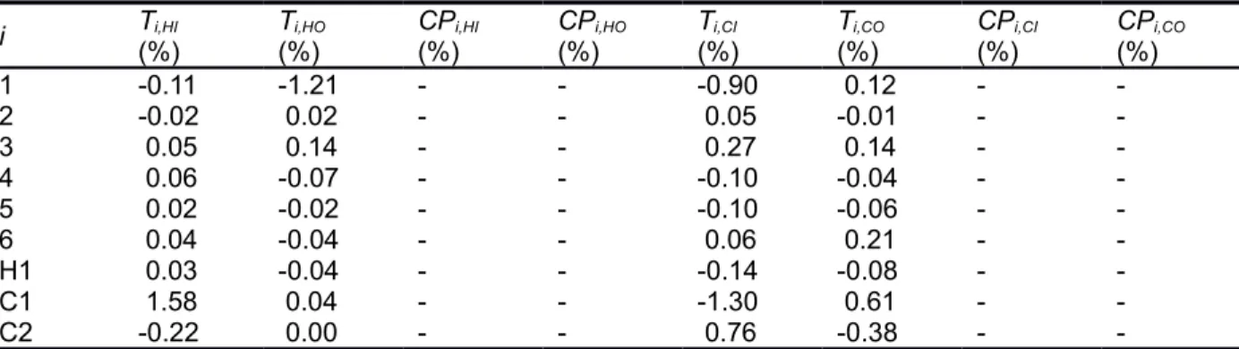
According to Step 6, the difference of the constant parameter in Step 4(a) (i.e. RT in Table 3.2) and obtained parameter in Step 5(a) (i.e. RT in Table 3.3) is calculated.
Table 3.4: Percentage difference of RT in first iteration for illustrative case study following CP path
i Ti,HI
(%) Ti,HO
(%) CPi,HI
(%) CPi,HO
(%) Ti,CI
(%) Ti,CO
(%) CPi,CI
(%) CPi,CO
(%)
1 -0.11 -1.21 - - -0.90 0.12 - -
2 -0.02 0.02 - - 0.05 -0.01 - -
3 0.05 0.14 - - 0.27 0.14 - -
4 0.06 -0.07 - - -0.10 -0.04 - -
5 0.02 -0.02 - - -0.10 -0.06 - -
6 0.04 -0.04 - - 0.06 0.21 - -
H1 0.03 -0.04 - - -0.14 -0.08 - -
C1 1.58 0.04 - - -1.30 0.61 - -
C2 -0.22 0.00 - - 0.76 -0.38 - -
From Table 3.4, it is shown that the differences are well below 2 %. Since in this case study the required satisfactory level is below 5 %, the results are accepted. For primary analysis, one round of iteration is sufficient to achieve the result and solve the data reconciliation problem. It can be further iterated to achieve stricter satisfactory level. To do so, according to Figure 3.5,
the next step is Step 5(b), where the obtained RT is kept constant and CP model is solved to obtain RCP.
Table 3.5: Result for the illustrative case study after Step 5(b) in second iteration following CP path
i Ti,HI
(°C) Ti,HO
(°C) CPi,HI
(kW/°C) CPi,HO
(kW/°C) Ti,CI
(°C) Ti,CO
(°C) CPi,CI
(kW/°C) CPi,CO
(kW/°C)
1 184.7 61.3 407.8 407.8 28.3 129.8 495.7 495.7
2 249.6 170.5 506.4 506.4 129.8 210.6 495.7 495.7
3 569.6 370.1 298.2 298.2 210.6 330.6 495.7 495.7
4 410.5 339.1 192.3 192.3 330.6 358.3 495.7 495.7
5 468.0 367.6 294.8 294.8 358.3 418.0 495.7 495.7
6 560.4 524.4 966.7 966.7 418.0 488.2 495.7 495.7
H1 800.4 699.9 294.5 294.5 488.2 547.9 495.7 495.7
C1 61.3 19.0 407.8 407.8 4.5 10.0 3,136.1 3,136.1
C2 370.1 319.5 298.2 298.2 5.0 9.9 3,079.3 3,079.3
After step 5(b), step 6 is visited again. The obtain RCP results in Table 3.5 are used to compare with the RCP results in Table 3.3. The differences are shown in Table 3.6. The calculated differences are around 1 %, which are lower than pervious iteration.
Table 3.6: Percentage difference of RCP in second iteration for illustrative case study following CP path
i Ti,HI
(%) Ti,HO
(%) CPi,HI
(%) CPi,HO
(%) Ti,CI
(%) Ti,CO
(%) CPi,CI
(%) CPi,CO
(%)
1 - - 1.27 1.27 - - 1.18 1.18
2 - - 1.06 1.06 - - 1.18 1.18
3 - - 1.20 1.20 - - 1.18 1.18
4 - - 1.35 1.35 - - 1.18 1.18
5 - - 1.00 1.00 - - 1.18 1.18
6 - - 1.21 1.21 - - 1.18 1.18
H1 - - 1.29 1.29 - - 1.18 1.18
C1 - - 1.27 1.27 - - -0.05 -0.05
C2 - - 1.20 1.20 - - -0.38 -0.38
To see how well the iterative method performs using CP path, the final result from Table 3.6 is compared with respective mean values in . Most of the reconciled parameters do not defer more than 2 % from mean values, with the highest being less than 4 %.
T path is to be demonstrated next to show the effect of choosing different part. After step 2, step 3(b) and 4(b) are to be followed next. While solving the T model, the mean values of CP parameters are substituted and kept constant. Table 3.8 shows the result after step 4(b).
Table 3.7: Percentage difference of the results obtained after second iteration for illustrative case study following CP path with respective mean values
i Ti,HI
(%) Ti,HO
(%) CPi,HI
(%) CPi,HO
(%) Ti,CI
(%) Ti,CO
(%) CPi,CI
(%) CPi,CO
(%)
1 -0.11 -1.21 1.71 1.98 -0.90 0.12 -0.45 -0.51
2 -0.02 0.02 0.98 1.11 0.05 -0.01 -0.87 -0.87
3 0.05 0.14 -0.97 -1.00 0.27 0.14 -0.79 -0.90
4 0.06 -0.07 -3.89 -3.93 -0.10 -0.04 -1.13 -0.94
5 0.02 -0.02 -1.51 -1.76 -0.10 -0.06 -0.75 -0.97
6 0.04 -0.04 -3.41 -3.38 0.06 0.21 -0.85 -1.06
H1 0.03 -0.04 -1.67 -1.81 -0.14 -0.08 -0.75 -0.78
C1 1.58 0.04 2.12 1.91 -1.30 0.61 -1.92 -1.97
C2 -0.22 0.00 -1.52 -1.00 0.76 -0.38 2.62 2.62
Table 3.8: Result for the illustrative case study after step 4(b) in first iteration following T path i Ti,HI
(°C) Ti,HO
(°C) CPi,HI
(kW/°C) CPi,HO
(kW/°C) Ti,CI
(°C) Ti,CO
(°C) CPi,CI
(kW/°C) CPi,CO
(kW/°C)
1 185.5 60.9 400.9 399.9 29.3 129.6 498.0 498.3
2 250.2 169.9 501.5 500.9 129.6 210.1 500.1 500.1
3 569.5 370.2 301.1 301.2 210.1 330.2 499.7 500.3
4 410.2 339.4 200.1 200.2 330.2 358.4 501.4 500.5
5 467.6 368.0 299.3 300.1 358.4 418.2 499.5 500.6
6 559.9 524.9 1,000.8 1,000.6 418.2 488.2 500.0 501.1
H1 800.2 700.1 299.5 299.9 488.2 548.2 499.5 499.7
C1 60.9 19.0 399.3 400.1 4.6 9.9 3,197.6 3,199.0
C2 370.2 319.5 302.8 301.2 4.9 10.0 3,000.6 3,000.6
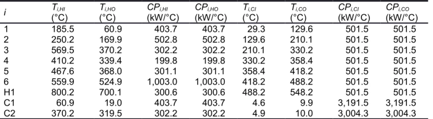
In step 5(b), using the result in Table 3.8, RT is kept constant and RCP is solved in CP model.
Table 3.9 shows the result after step 5(b).
Table 3.9: Result for the illustrative case study after step 5(b) in first iteration following T path i Ti,HI
(°C) Ti,HO
(°C) CPi,HI
(kW/°C) CPi,HO
(kW/°C) Ti,CI
(°C) Ti,CO
(°C) CPi,CI
(kW/°C) CPi,CO
(kW/°C)
1 185.5 60.9 403.7 403.7 29.3 129.6 501.5 501.5
2 250.2 169.9 502.8 502.8 129.6 210.1 501.5 501.5
3 569.5 370.2 302.2 302.2 210.1 330.2 501.5 501.5
4 410.2 339.4 199.8 199.8 330.2 358.4 501.5 501.5
5 467.6 368.0 301.1 301.1 358.4 418.2 501.5 501.5
6 559.9 524.9 1,003.0 1,003.0 418.2 488.2 501.5 501.5
H1 800.2 700.1 300.6 300.6 488.2 548.2 501.5 501.5
C1 60.9 19.0 403.7 403.7 4.6 9.9 3,191.5 3,191.5
C2 370.2 319.5 302.2 302.2 4.9 10.0 3,004.3 3,004.3
According to Step 6, the difference of the constant parameter in Step 4(b) (i.e. RCP in Table 3.8) and obtained parameter in Step 5(b) (i.e. RCP in Table 3.9) is calculated. The results are shown in Table 3.10.
Table 3.10: Percentage difference of RCP in the first iteration for illustrative case study following T path
i Ti,HI
(%) Ti,HO
(%) CPi,HI
(%) CPi,HO
(%) Ti,CI
(%) Ti,CO
(%) CPi,CI
(%) CPi,CO
(%)
1 - - 0.70 0.96 - - 0.70 0.64
2 - - 0.25 0.38 - - 0.28 0.28
3 - - 0.37 0.34 - - 0.36 0.25
4 - - -0.17 -0.22 - - 0.02 0.21
5 - - 0.60 0.35 - - 0.40 0.18
6 - - 0.22 0.25 - - 0.30 0.09
H1 - - 0.37 0.23 - - 0.40 0.37
C1 - - 1.10 0.90 - - -0.19 -0.23
C2 - - -0.19 0.34 - - 0.12 0.13
From Table 3.10, the differences are mostly well below 1 %. As the differences are lower than the satisfactory level of 5 %, it shows that for this case study, T path is more suitable in this reconciliation problem. A round of iteration is sufficient to achieve the satisfactory result. Further iteration is carried out to check the performance of T path in this case study. According to Figure 3.5, the next step is Step 5(a), where the obtained RCP is kept constant and T model is solved to obtain RT.
Table 3.11: Result for the illustrative case study after Step 5(a) in second iteration following T path
i Ti,HI
(°C) Ti,HO
(°C) CPi,HI
(kW/°C) CPi,HO
(kW/°C) Ti,CI
(°C) Ti,CO
(°C) CPi,CI
(kW/°C) CPi,CO
(kW/°C)
1 185.5 60.9 403.7 403.7 29.3 129.6 501.5 501.5
2 250.2 169.9 502.8 502.8 129.6 210.1 501.5 501.5
3 569.5 370.2 302.2 302.2 210.1 330.2 501.5 501.5
4 410.2 339.4 199.8 199.8 330.2 358.4 501.5 501.5
5 467.6 368.0 301.1 301.1 358.4 418.2 501.5 501.5
6 559.9 524.9 1,003.0 1,003.0 418.2 488.2 501.5 501.5
H1 800.2 700.1 300.6 300.6 488.2 548.2 501.5 501.5
C1 60.9 19.0 403.7 403.7 4.6 9.9 3,191.5 3,191.5
C2 370.2 319.5 302.2 302.2 4.9 10.0 3,004.3 3,004.3
Following Step 6, the obtained RT results in Table 3.11 are used to compare with the kept constant RT results in Table 3.9. The calculated differences are shown in Table 3.12. All calculated differences are near to 0 %, with the highest value not exceeding 1 %. Further iteration is not required as it will produce similar result.
Table 3.12: Percentage difference of RT in second iteration for illustrative case study following T path
i Ti,HI
(%) Ti,HO
(%) CPi,HI
(%) CPi,HO
(%) Ti,CI
(%) Ti,CO
(%) CPi,CI
(%) CPi,CO
(%)
1 0.00 -0.01 - - 0.01 0.00 - -
2 0.00 0.00 - - 0.00 0.00 - -
3 0.00 0.00 - - 0.00 0.00 - -
4 0.00 -0.00 - - 0.00 -0.01 - -
5 -0.01 0.01 - - -0.01 0.01 - -
H1 0.00 0.00 - - 0.00 -0.00 - -
C1 -0.01 0.02 - - -0.71 0.33 - -
C2 0.00 0.00 - - 0.16 -0.08 - -
To see how well the iterative method performs using CP path, the final result in Table 3.12 is compared with respective mean values. Table 3.13 shows the calculated difference with respective mean values. Most of the difference values are not more than 2 %, with only one value not exceeding 2.5 %. This shows that T path is more suitable to be used in this case study, as reconciled parameters do not deviate from mean values compared to CP path.
Overall, it shows that iterative method, whether CP path or T path, is suitable to be used to obtain reconciled parameters in this case study. The possible difference between the CP path and T path is the initial parameters to be reconciled, as CP model involves lower number of parameters than T model. When compared to respective mean values, the differences have low values in an iteration. As for computational effort, since this case study is smaller scale in comparison, the results are obtained in less than 1 s.
Table 3.13: Percentage difference of the results obtained after second iteration for illustrative case study following T path with respective mean values
i Ti,HI
(%)
Ti,HO
(%)
CPi,HI
(%)
CPi,HO
(%)
Ti,CI
(%)
Ti,CO
(%)
CPi,CI
(%)
CPi,CO
(%)
1 0.31 -1.83 0.70 0.96 2.45 0.00 0.70 0.64
2 0.24 -0.36 0.25 0.38 -0.08 -0.22 0.28 0.28
3 0.03 0.15 0.37 0.34 0.06 0.04 0.36 0.25
4 -0.03 0.04 -0.17 -0.22 -0.21 0.00 0.02 0.21
5 -0.06 0.08 0.60 0.35 -0.05 -0.02 0.40 0.18
6 -0.06 0.06 0.22 0.25 0.10 0.20 0.30 0.09
H1 0.01 -0.01 0.37 0.23 -0.15 -0.01 0.40 0.37
C1 0.94 0.00 1.10 0.90 0.04 -0.02 -0.19 -0.23
C2 -0.20 0.00 -0.19 0.34 -1.96 1.00 0.12 0.13