UPON-2018 MANUSCRIPT: SPECTRAL ANALYSIS OF FLUCTUATIONS IN HUMANS’ DAILY MOTION USING LOCATION DATA

(1)

Fluctuation and Noise Letters Vol. 0, No. 0 (0000) 000–000

UPON-2018 MANUSCRIPT: SPECTRAL ANALYSIS OF FLUCTUATIONS IN HUMANS’ DAILY MOTION USING LOCATION DATA

GERGELY VADAI⁽¹⁾, ANDRÁS ANTAL⁽¹⁾ AND ZOLTÁN GINGL⁽¹⁾

(1) Department of Technical Informatics, University of Szeged, Szeged 6720, Hungary e-mail address: vadaig@inf.u-szeged.hu, antal.andras@stud.u-szeged.hu, gingl@inf.u-szeged.hu

Received (received date) Revised (revised date) Accepted (accepted date)

The interpretation and characterization of universal scaling laws in human mobility and activity are subjects of active research. For the better understanding, instead of the statistical approach we have examined the temporal patterns of human daily motion using location data. The trajectories were measured continuously and with even sampling (1 measurement per minute), using GPS and Wi-Fi/mobile internet signals of the participant’s smartphone. We have analyzed the few week-long signals of displacements between two subsequent samplings in frequency domain. Our results had shown, that 1/f type noise is observable over the frequency of the daily rhythm of motion and its harmonics. We point out several technical questions about the measurement and data processing required for further detailed analysis. Furthermore, our new observation could help in the investigation of the underlying dynamics of human motion and opens several theoretical questions about the relationship between the spatial and temporal universality.

Keywords: Human mobility; 1/f noise; human dynamics; GPS location data.

1. INTRODUCTION

The spatial and temporal patterns of human dynamics and its scale-free nature are subjects of active research in multidisciplinary fields.

The investigation of human mobility is based on the determination of location using direct or indirect methods i.e. GPS and Wi-Fi signals, phone calls, banknote dispersal, check-ins in web applications or usage of social media [1-5]. After the pioneer studies had shown that animals wandering are not Brownian motion but Lévy-flight [6,7], statistical investigation of individual human trajectories and understanding the underlying dynamics came into the spotlight in the last decade. The displacements and waiting times of human dynamics follow non-Poisson statistics, however several effects like the population’s het- erogeneity and the motions spatial and temporal regularity make the interpretation and characterization of the observed heavy-tailed distributions more difficult, moreover, the different methods used for monitoring locations could affect the result of the analysis [2,4].

Numerous measurements and studies led to different conclusions for the scaling laws and models of mobility [1-5,8-15].

Fluctuation and Noise Letters VOL. 18, NO. 02, 2019, 1940010 https://doi.org/10.1142/S0219477519400108

(2)

The analysis of human motion in time domain can be based on the measurement of activity using inertial sensors. The signals of actigraphs mounted on the human body (most often on the wrist) are useful at monitoring rest/activity cycles and in the diagnosis of sleep or several mental disorders [16]. The analysis of the daily activity patterns helped to find universal distribution laws of human behavior; the resting periods follow scale-invariant power law [16,17]. Furthermore, over the frequency region of circadian rhythm and its harmonics, 1/f type noise is observable in the power spectral density of activity signals [17].

In the analysis of human behavior, the spatial and temporal regularity must be taken into consideration [4,11,14]. For better understanding, instead of the statistical analysis, we have examined the temporal patterns of individual motion – which is a rarely used approach [14] – and have collected the location data likewise actigraph signals. Based on the measurements we have conducted using smartphones, we have observed 1/f type noise over the frequency region of the daily rhythm of motion, however the inevitable measurement errors and the difficulties of the analysis of signals brought up technical problems. Nevertheless, the scale-free nature of human behavior predicted in the frequency domain could throw new light upon the research of mobility, from which numerous open question emerge.

2. MEASUREMENT OF LOCATION DATA

For the spectral analysis of the temporal patterns observed in humans’ daily motion, we studied the displacements between two subsequent measured positions as an activity-like quantity. For this, unlike previous studies, the measurement should be uniformly sampled and its sampling frequency needed to be much higher than the frequencies used in most of the previous studies. Furthermore, the measurement time period needed to be longer, several days or weeks long.

Since the location data of available databases or data measured by commercial GPS loggers do not meet the mentioned three requirements simultaneously, we conducted a 3- week long measurement using a smartphone application specially developed to log the users’ location data. This application recorded the GPS and Wi-Fi/mobile internet signals of the user’s smartphone with a sample rate of 1 measurement per minute and collected them in a server. The advantage of this solution is that, when the user is in a building or any kind of vehicle, the location data can be recorded through the Wi-Fi or mobile internet signal.

However, the optimal energy usage and the operating system’s application priority settings caused errors make the measurement procedure’s implementation a great challenge due to the used different devices and Android versions.

3. SIGNAL PROCESSING

Because of the mentioned problems, the required long and uniformly sampled measurement is impossible without losing some data points. Furthermore, the location accuracy of the commercially available GPS modules is limited, and the measured data could also con- tain some false data points.

In most of the cases, the cause of these false data points was one of three error types we found during the analysis. First, the Android operating system’s priority policy can cause the measurement application to shut down or its measurement to be incorrect, caus- ing missing or false data points. This error causes the data to be either missing, or the GPS module falsely registers the user to be at the 0,0,0 GPS coordinate. Second, the commercially available GPS modules’ accuracy can differ, depending on the available satellites.

As a result, data points can be greatly inaccurate. This error usually come up, when the

(3)

user is inside a building. Third, the device’s GPS module can lose its signal when it is inside a vehicle. Using any kind of transportation, the vehicle can block out the GPS signal and, as a result, the application registers the last “known” location with an increasing accuracy value until the user exits the vehicle.

As we can see, the prudent analysis of the measured data and its cleaning is definitely required. Also, the tracking of the effects of these and the exclusion of the possible artefacts is especially important in the appropriate interpretation of the results.

The salient longitude and latitude data points and displacement values, often the effect of using public transportation or travel via car, are being deleted. An important question in the course of analysis is the impact of the intervention, for example a longer travel’s dele- tion can exclude a “big wander” which can damage the motion’s suspected Lévy-flight like nature [18].

Therefore, the motion of 17 users’ data analyzed below were categorized by the amount of missing or deleted data points. In addition, the analysis presented below has been made using different preprocessing methods and the results have been compared.

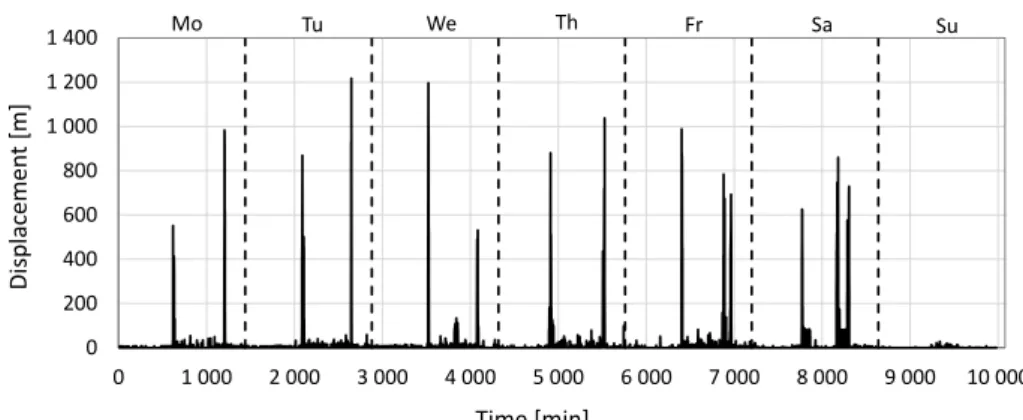
In Fig. 1. an example of a user’s displacement values of one week can be seen. In the figure the daily schedule of the user – for example its travel to and from workplace – can be observable in the weekdays and the motion differs clearly on Sunday.

Fig. 1. Minutely displacement values of the measurement’s first week of a participant and markers for each day.

Fig. 2. Zipf plot of visit frequencies of a participant’ motion for the whole 3-week long period. The number of visiting a location plotted in the function of the locations’ rank listed in the order of the number of visits.

0 200 400 600 800 1 000 1 200 1 400

0 1 000 2 000 3 000 4 000 5 000 6 000 7 000 8 000 9 000 10 000

Displacement [m]

Time [min]

Mo Tu We Th Fr Sa Su

1 10 100 1 000 10 000

1 10 100

Number of visits

Rank

(4)

For the detailed characterization of human mobility patterns, much more participant’s statistical analysis is required. However, in Fig. 2., the scale-invariant nature of one participant’s motion is demonstrated clearly, the frequency of visiting different locations follows a power-law as it was presented in previous studies with the analysis of large populations [2]. This Zipf plot depicts clearly that the individual revisits a few locations frequently, which can be explained by its daily routine.

4. SPECTRAL ANALYSIS

The classical Fourier analysis of the measured minutely displacement – in other words, velocity – signals is not possible directly due to the deleted or missing data points. To eliminate the problem of unevenly sampled data, we used the Lomb periodogram [19] for the analysis of the power spectral density (PSD).

In the case of 4 individuals the 3-week long measurement more than 95% of the data could be retained and in the case of additional 1 user still more than 85% could be used.

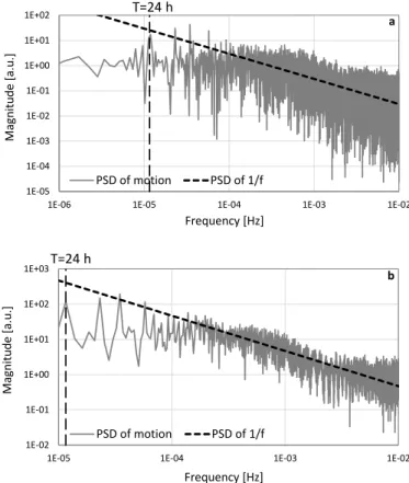
The PSD of these signals for the whole time window was similar in shape as can be seen in Fig. 3.a: peaks can be observed at the frequency belongs to the one-day period (1,157 ∙ 10^-5 Hz), and at its harmonics. Above this region of daily rhythm of motion, 1/f type noise is observable over a corner frequency.

Fig. 3. Lomb periodogram of a participant’s motion (displacements per 1 minute) for the whole 3-week long period (a) and the average of the 1-week long periods (only weekdays) (b). The PSD of 1/f noise is also depicted for illustration with dashed line.

1E-05 1E-04 1E-03 1E-02 1E-01 1E+00 1E+01 1E+02

1E-06 1E-05 1E-04 1E-03 1E-02

Magnitude [a.u.]

Frequency [Hz]

PSD of motion PSD of 1/f T=24 h

a

1E-02 1E-01 1E+00 1E+01 1E+02 1E+03

1E-05 1E-04 1E-03 1E-02

Magnitude [a.u.]

Frequency [Hz]

PSD of motion PSD of 1/f T=24 h

b

(5)

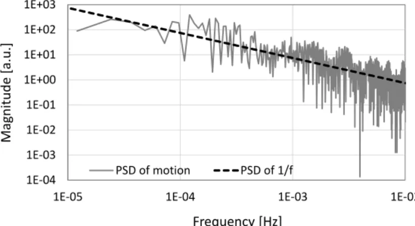
This nature can be detected more accurately in the averaged PSD-s of the first two week’s weekday periods of the same motion, as can be seen in Fig. 3.b. In the case of the above mentioned 5 users’ signals, the fitting of 1/f^α curve’s α value is between 0,85 and 1,15 for the whole, weekly or daily averaged spectra and for different fitting parameters, too. An example of the daily averaged spectrum can be seen in Fig. 4., where we used 14 days from a participant’s data.

Fig. 4. Averaged spectrum of a participant’s motion (displacements per 1 minute) of one-day long periods for 14 days of measurement and the PSD of 1/f noise illustrated with dashed line.

In the case of 12 individuals, data are missing at several, longer time intervals because of the mentioned measurement errors or removal of false data points. However, the remain- ing periods’ PSD and shorter – even few-hour long – signal pieces’ averaged spectra had shown the same nature in the mentioned frequency domain. The fitting 1/f^α curve’s α value varies between 0,8 and 1,3. Examples can be seen for these cases in Fig. 5., where a one- day long measurement of an aforementioned individual’s motion is shown, and Fig. 6., which is an example of the averaged spectrum of a participant’s data. In this latter case, the spectra were calculated for the time window between 6 AM and 4 PM in every day for a four-day long period.

Fig. 5. Lomb periodogram of a participant’s motion (displacements per 1 minute) for one day. PSD of 1/f noise is also depicted for illustration with dashed line.

1E+00 1E+01 1E+02 1E+03 1E+04

1E-05 1E-04 1E-03 1E-02

Magnitude [a.u.]

Frequency [Hz]

PSD of motion PSD of 1/f

1E-04 1E-03 1E-02 1E-01 1E+00 1E+01 1E+02 1E+03

1E-05 1E-04 1E-03 1E-02

Magnitude [a.u.]

Frequency [Hz]

PSD of motion PSD of 1/f

(6)

Fig. 6. Averaged spectrum of a participant’s motion (displacements per 1 minute) for the time window between 6 AM and 4 PM in every day for a four-day long period. PSD of 1/f noise is also depicted for illustration with dashed line.

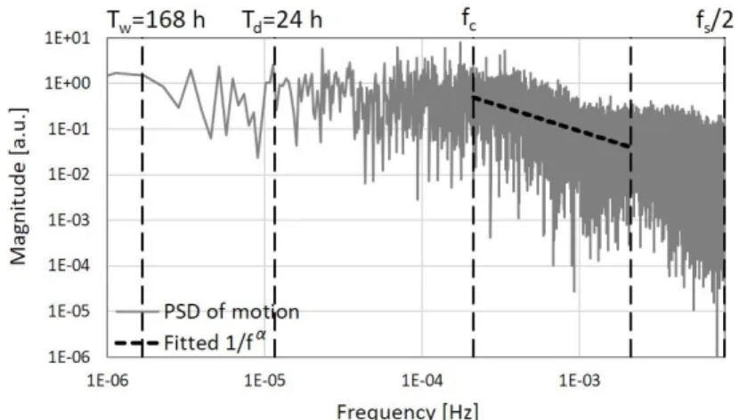
As it depicted in Fig. 7., a typical structure of the spectrum can be described as follows:

peaks can be found at the frequencies belonging to the one-week and one-day period (Tw

and Td). After this region and above a corner frequency (fc), presence of 1/f^αtype noise is observable. This nature is similar to what was previously found in the case of activity signals [8].

However, several conditions can make the fitting required to calculate the α value more difficult: we have limited information about the corner frequency’s accurate value, it has been changing around the 1-hour period’s frequency value. The analysis we conducted on all, 17 users’ data shows that value of fc is constant for each individual, regardless of the used time window and varies slightly for different participants. Furthermore, because of these values, the possibility of the aliasing at high frequencies and the sampling frequency (fs), which cannot be easily increased further in case of smartphone measurements, the noise can only be examined over 1-2 decades.

Fig. 7. Lomb periodogram of a participant’s motion (displacements per 1 minute) for the whole 3-week long period with markers for frequencies belonging to the weekly period (Tw), daily period (Td) and the corner frequency (fc).

(7)

For the confirmation that this new result, the 1/f noise’s presence, is due to the human behavior and not caused by the measurement process or the preprocessing, we compared the results for every user in several different manners and numerous time windows. Neither the different removal rules – for example removing every displacement greater than a given threshold –, nor the signal’s under-sampling – namely resampling the signals with a lower sample rate thus eliminating the effect of missing data points – didn’t show significant difference, 1/f type noise is observable for all of the 17 participants.

To be certain that the accuracy of the used GPS modules did not affect the spectral shape of the motion, the original data was modulated with Gaussian white noise with a standard deviation similar in value to the module’s accuracy value. The characteristics of the resulting spectra and the spectra of the original data were indistinguishable.

Furthermore, we examined the possibility of replacing the missing data points, and use Discrete Fourier transform (DFT) to calculate the PSD instead of the Lomb periodogram.

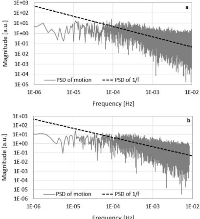
In the case of the 3-week long signals, replacing the missing data points with the last known location or the linear interpolation of the missing periods had shown the same results as the original signal’s PSD. In Fig. 8.b, the rate of missing points from a participant’s data were only ~3%, in Fig. 9.b, in a case of another individual it was ~33%, and these points were replaced using linear interpolation. These spectra show highly similar shape as the Lomb periodograms depicted in Fig. 8.a, and Fig. 9.a. However, this method’s reliability and usability brings up additional technical questions when there are more false data points.

Fig. 8. Lomb periodogram (a) and Fourier-based PSD (b) of a participant’s motion (displacements per 1 minute) for the whole 3-week long period after replacement of the missing data using linear interpolation (nearly 900 missing points). PSD of 1/f noise is also depicted for illustration with dashed line.

(8)

Fig. 9. Lomb periodogram (a) and Fourier-based PSD (b) of a participant’s motion (displacements per 1 minute) for the whole 3-week long period after replacement of the missing data using linear interpolation (nearly 9900 missing points). PSD of 1/f noise is also depicted for illustration with dashed line.

5. CONCLUSION AND OPEN PROBLEMS

Through the measurement of humans’ location data and the analysis of their minutely displacement, we have observed 1/f type noise over a corner frequency, above the frequency range of the daily rhythm of motion. This prediction and the method of using spectral analysis could be useful in the examination of the effects of temporal regularity, caused by the circadian rhythm and in the characterization of the random motion at higher frequencies. On the other hand, as we pointed out, the implementation of the required large, long term, evenly sampled measurements and the appropriate preprocessing of the data raise several technical questions. For the better understanding of the phenomenon, the determination of the α value and to study the effect of the different conditions (temporal and spatial regularity caused by the nature of the individual’s profession, age, health condition etc.) more measurements and detailed analysis are required.

The presence of 1/f type noise in humans’ daily motion raises several, interesting theoretical questions: what is the source of the noise? How could we describe it with the actual mathematical models of human mobility or how it could be integrated to them? What is the relationship between the displacements’ distribution and its scale-free nature in frequency domain?

(9)

The motion’s power spectral density is divided by the corner frequency to two separate elements: a white noise, containing the motion’s circadian rhythm and its harmonics, which appears at lower frequencies and a 1/f^α noise at the higher frequencies. Further open question is the value of the α: for some cases, possibly other values could describe the phenomenon, for example 1.5 corresponding to diffusion noise [20].

Therefore, the observation of 1/f type noise over a corner frequency and the investigation of the above mentioned unsolved problems could help in the theoretical investigation of the underlying dynamics of human behavior and in the explanation of scaling laws of human activity and mobility.

ACKNOWLEDGEMENTS

The authors thank Ferenc Lakos and Dániel Vince for their assistance making the smartphone application for the measurements. Discussions with Róbert Mingesz about measurement techniques and spectral analysis are greatly appreciated.

This research was supported by the Hungarian Government and the European Regional Development Fund under the grant number GINOP-2.3.2-15-2016-00037 (“Internet of Living Things”).

References

[1] D. Brockmann, L. Hufnagel, T. Geisel, “The scaling laws of human travel”, Nature 439, (2006) 462–465.

[2] M. C. González, C. A. Hidalgo, A. L. Barabási, “Understanding individual human mobility patterns” Nature 453 (2008), 779-782.

[3] C. M. Song, T. Koren, P. Wang, et al., “Modelling the scaling properties of human mobility”, Nature Physics 6 (2010), 818–823.

[4] L. Alessandretti, P. Sapiezynski, S. Lehmann, et al., “Multi-scale spatio-temporal analysis of human mobility”, PLoS ONE 12 (2017), e0171686.

[5] R. Jurdak, K. Zhao, J. Liu, M. AbouJaoude, M. Cameron, D. Newth, “Understanding Human Mobility from Twitter”, PloS ONE, 10 (7) (2015), e 0131469.

[6] G. M. Viswanathan, V. Afanasyev, S. V. Buldyrev, et al., “Lévy flight search patterns of wandering albatrosses”, Nature 381 (1996), 413 - 415.

[7] D. W. Sims, E. J. Southall1, N. E. Humphries, et al., “Scaling laws of marine predator search behavior”, Nature 451 (2008), 1098–1102.

[8] I.Rhee, M. Shin, S. Hong, K. Lee, S. Chong, „On the Levy-walk Nature of Human Mobility:Do Humans Walk like Monkeys?”, IEEE/ACM Transactions on Networking (TON) 3(19) (2011), 630-643

[9] S. Petrovskiia, A. Mashanovab, V. A. A. Jansen, “Variation in individual walking behavior cre- ates the impression of a Lévy flight”, PNAS 108(21) (2011), 8704-8707

[10] K. Zhao, M. Musolesi, P. Hui, W. Rao, S. Tarkoma, “Explaining the power-law distribution of human mobility through transportation modality decomposition”, Scientific Reports 5 (2015), 9136

[11] CM Schneider, V Belik, T Couronné, Z Smoreda, MC González, “Unravelling daily human mobility motifs.”, Journal of The Royal Society, Interface 10(84) (2013), 20130246

[12] H. Liu, YH. Chen, JS. Lih, “Crossover from exponential to power-law scaling for human mobility pattern in urban, suburban and rural areas”, The European Physical Journal B 88(117) (2015)

[13] R. Gallotti, A. Bazzani, S. Rambaldi, M. Barthelemy, “A stochastic model of randomly accel- erated walkers for human mobility”, Nature Communications 7(12600) (2016)

[14] XW. Wang, XP. Han, BH. Wang, “Correlations and Scaling Laws in Human Mobility”, PLoS ONE 9 (1) (2014), e84954

(10)

[15] L. Alessandretti, P. Sapiezynski, S. Lehmann, A. Baronchelli, “Multi-scale spatio-temporal analysis of human mobility”, PloS ONE, 12 (2) (2017), e0171686.

[16] T. Nakamura, K. Kiyono, K. Yoshiuchi, et al., “Universal Scaling Law in Human Behavioral Organization”, Physical Review Letters 99 (2007), 138103.

[17] J. K. Ochab, J. Tyburczyk, E. Beldzik, et al., “Scale-Free Fluctuations in Behavioral Perfor- mance: Delineating Changes in Spontaneous Behavior of Humans with Induced Sleep Defi- ciency”, PLoS ONE 9 (2014), e107542.

[18] A. M. Edwards, R. A. Philips, N. W. Watkins, M. P. Freeman, E. J. Murphy, V. Afanasyev, S.

V. Buldyrev, M. G. E. da Luz, E. P. Raposo, H. E. Stanley, G. M. Viswanathan, “Revisiting Lévy flight search patterns of wandering albatrosses, bumblebees and deer”, Nature 449 (2007), 1044–

1048.

[19] N. R. Lomb, “Least-squares frequency analysis of unequally spaced data”, Astrophysics and Space Science 39 (1976), 447–462.

[20] G. Schmera, L. B. Kish, “Surface diffusion enhanced chemical sensing by surface acoustic waves”, Sensors and Actuators B: Chemical, 93 (2003), 1-3