CYCLE INTEGRALS OF MODULAR FORMS DISSERTATION submitted for the degree of “Doctor of the Hungarian Academy of Sciences” Árpád Tóth Eötvös Loránd University

(1)

CYCLE INTEGRALS OF MODULAR FORMS

DISSERTATION submitted for the degree of

“Doctor of the Hungarian Academy of Sciences”

Arp´ ´ ad T´ oth

E¨ otv¨ os Lor´ and University

and

MTA Alfr´ed R´enyi Institute of Mathematics

Budapest

2018

(2)

(3)

Introduction

The goal of this dissertation is to describe some new results on the integrals of modular forms along certain closed curves. We will refer to these integrals as cycle integrals of modular forms. When interpreted classically the curves of integration are closed geodesics on the so called modular surface, the quotient of the hyperbolic plane of Bolyai-Lobachevsky by a distinguished discrete group of isometries. In this language the simplest modular forms are eigenfunctions of the Laplace-Beltrami operator. However for certain applications it is better to view them as functions on PSL2(R) the isometry group of the hyperbolic plane.

In this version modular forms have a natural representation theoretic interpretation. The lift of closed geodesics then become periodic orbits of the geodesic flow, and the integral of modular forms along them give interesting information about these periodic orbits, such as their linking numbers.

For example when the discrete group in question is SL₂(Z), the right-coset space SL2(Z)\SL2(R) as a 3-manifold is diffeomorphic to the complement of the trefoil knot in S³, as realized as the link of the surface singularity of z² =w³ at the origin. E. Ghys showed that the linking number of this trefoil knot with a periodic orbit of the geodesic flow (called a modular knot in this case) is given by the Rademacher symbol. This symbol is a close relative of the classical Dedekind symbol which arose historically in the computation of cycle integrals of the logarithmic derivative of Dedekind’s eta function. In his 2006 ICM talk Ghys brought attention to the intriguing question of understanding linking numbers between modular knots either combinatorially or from an arithmetic point of view. These linking numbers have to be properly interpreted asH₁(S³\Trefoil) =Z. A natural path to take is to consider the symmetrized link of a modular knot, these arise as the union of the periodic orbits corresponding to some γ, γ⁻¹ ∈SL₂(Z). One of the problems considered in this thesis concerns the construction of analogues of Dedekind’s eta function whose cycle integrals produce the linking numbers between these symmetrized links. This is Chapter 5 of the present thesis, based on the paper [42].

Another interesting application of cycle integrals presented in this dissertation concerns mock modular forms. Their theory was outlined by Ramanujan in his last letter to Hardy, a few month before his untimely death at age 32. It was only recently in 2002 that Zwegers found an intrinsic description of the elusive idea of what Ramanujan’s mock modular forms are. Surprisingly, cycle integrals of PSL2(Z)-invariant functions with respect to arc length give a natural construction of these objects [40]. This material is presented in Chapter 4.

There is yet another problem that arose recently concerning immersed surfaces on the modular surface whose boundary is one of the closed geodesics. It is natural to expect that the push-forward measure of the natural hyperbolic metric on these surfaces gets equidis- tributed as the discriminant (a natural invariant of the geodesics) approaches infinity. This problem too leads to cycle integrals, this time of PSL2(Z)-invariant differential forms, and require a generalization of formulas due to Maass, and Katok-Sarnak [43]. This general-

(6)

ization and the resulting equidistribution results are presented from [43] and they form Chapters 2 and 3 of the thesis.

Finally cycle integrals are closely related to sums of certain exponential sums named after Salie and this is what we consider in the last chapter. This has interesting applications to the equidistribution of the so-called angles of these sums, or equivalently to the distribution of the roots of quadratic congruences to prime moduli. A conceptual background for why one expects such equidistribution is given for example in [112]. The major result of this chapter is from [123], which establishes these equidistribution results.

We will now put the results presented here in the framework of recent advances in automorphic forms. This thesis deals with generalizations of work of Katok, Sarnak, Borcherds, Zagier, Ghys, and many others and leads to some surprising new applications. It is without doubt that for the general public the most exciting new developments in modular form theory are related to Langland’s program on the relation between automorphic forms and Galois representations. Instances such as Lafforgue’s proof of the Langlands’ conjectures for the general linear group GL(n, K) for function fields or Ngo’s proof of the fundamental lemma for general reductive groups received Fields medals. (Lafforgue’s work contin- ued earlier research of Drinfeld, another Fields medalist, who treated the case GL(2, K).) Widely known by the general public is Wiles’ work on the modularity of Galois representations associated to elliptic curves that allowed him to prove Fermat’s last theorem.

Borcherds’ achievements for which he too was awarded a Fields medal were more con- nected to classical modular forms. Another major development is Lindenstrauss proof of the quantum unique ergodicity (QUE) conjecture of Rudnick and Sarnak for arithmetic surfaces for which he received the Fields medal in 2010. Also highly praised is this year’s Fields medalist Venkatesh’ work that very successfully brought in homogeneous dynamics into the subject. In both Lindenstrauss’ and Venkatesh’ work the role of number theory, while somewhat hidden, is significant. The research presented in this thesis is in different directions but in the same vain as theirs. Analysis and geometry in the classical sense play a more accentuated role than number theory but arithmetic considerations are crucial in most of the results presented below.

The organization of the dissertation is as follows. Chapter 1 gives a very short introduction to modular forms to set up notation. In Chapter 2 we develop a formalism to deal with cycle integrals of Poincar´e series, this formalism will be used on several occasions.

The first of these applications is this same chapter’s main result about the extension of the Katok-Sarnak formulas taken from [43]. Chapter 3 is about the resulting two-dimensional equidistribution problem from [43]. Chapter 4 gives a brief description of mock modular forms and describes how these can be constructed from cycle integrals [40]. It also includes a construction of certain modular integrals used in connection with linking numbers in the chapter that follows. In that chapter, Chapter 5, we review Ghys’ work on the geodesic flow and derive our results from [42] on linking numbers between symmetrized modular knots. Finally we prove the equidistribution of the angles of Salie sums in Chapter 6 [123].

(7)

Chapter 1 Background on modular forms

1.1 Hyperbolic geometry in the upper half plane model

One of the major discoveries of J´anos Bolyai [56] was the fact that hyperbolic space contains a surface (the so called parasphere or horopsphere) on which the natural geometry satisfies the axioms of Euclid. Beltrami observed that the projection of a hyperbolic plane to this surface gives models of hyperbolic geometry on an open disc in the Euclidean plane.

One of these models is conformal, and can be taken to the upper half plane via Cayley’s transformation. This model was rediscovered and popularized by Poincar´e while working on Fuchsian funtions, and is usually named the Poincar´e upper half plane [121].

Let H={z ∈C: Imz >0}. The group

GL⁺₂(R) = {[^{a b}_{c d}] : a, b, c, d∈R, ad−bc >0}

acts on Cvia M¨obius transformations, for g = [^{a b}_{c d}]∈GL⁺₂(R) gz = az+b

cz+d.

If z ∈ H then Imgz = detg_|cz+d|^Im^z2 and so gz is also in H. One checks easily that this is a left action of GL⁺₂(R) on H, (g₁g₂)(z) = g₁(g₂(z)). By an easy application of Swartz’s lemma one sees that all holomorphic automorphisms ofH are given by such M¨obius transformations. These automorphisms as a group are easily seen to be isomorphic to PSL₂(R).

The metric

ds² = 1

y²(dx²+dy²)

is invariant under the action of PSL₂(R) (and has constant curvature -1). It follows that the conformal isomorphisms are the orientation preserving isometries.

One verifies easily that vertical lines are geodesics, and then so are their PSL₂(R)- translates, which lead to semi-circles whose center lies on the real line. These are then the hyperbolic lines of the model.

Define the cross ratio of z₁, z₂, z₃, z₄ ∈Cby

[z₁, z₂, z₃, z₄] = (z₁−z₃)(z₂−z₄)

(z₁−z₂)(z₃−z₄). (1.1.1)

(8)

A useful formula for the distance between z and z^∗ inH is given by

d(z, z^∗) = log|[w, z, z^∗, w^∗]|, (1.1.2) where w, w^∗ ∈ R are the points where the geodesic arc joining z to z^∗ intersects R and where the order in which this arc passes through the points is given byw, z, z^∗, w^∗ (see e.g.

[9]).

If d(z, w) is the distance, then in terms of Cartesian coordinates it is easier to work with

coshd(z, w) = 1 + 2u(z, w) where

u(z, w) = |z−w|² 4 ImzImw

The measure associated to the metric is also invariant and is given by µ= dxdy

y²

The hyperbolic Laplace operator is defined on smooth functions as the operator

∆ = (∆H) = y²(∂_x²+∂_y²) = (y²∆_R²).

One can show that −∆ is a non-negative operator on various L²-spaces (see below), and so the normalization of the eigenvalues is as follows. If

∆f +λf = 0

then we callλ an eigenvalue. With this understanding the eigenvalues that arise for us are non-negative and we can write them using additional parameters:

λ= 1

4+r² =s(1−s).

Here r∈R orir ∈[−¹₂,¹₂] and s= ¹₂ +ir. So eachλ 6= ¹₄ corresponds to two r values ±r, and two s values s= ¹₂ ±ir.

1.2 SL

₂

( Z )

Let Γ =P SL₂(Z), it is a discrete subgroup of PSL₂(R) and so acts totally discontinuously on H. From the Euclidean algorithm or otherwise one shows that Γ = hS, Ti, where as M¨obius transformations S(z) = −¹_z and T(z) =z + 1. We will occasionally overload the notation by identifying S and T with the matrices

S = [⁰_{1 0}⁻¹] and T = [^{1 1}_{0 1}] or their image in PSL₂(Z).

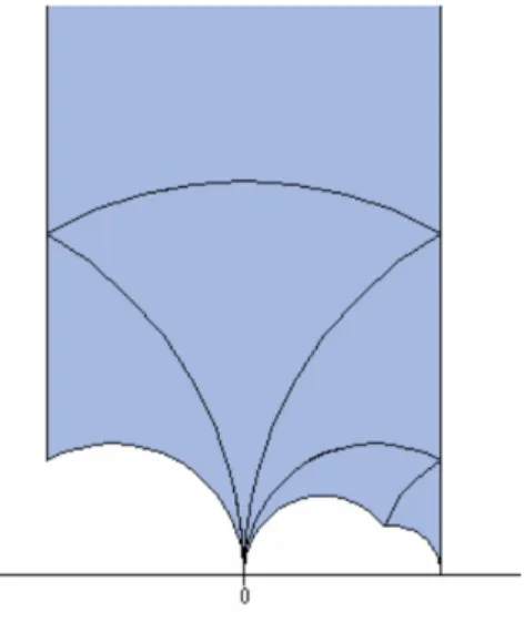
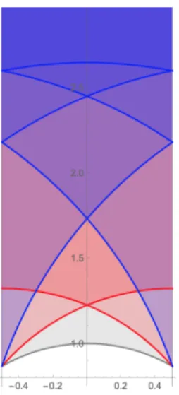
A fundamental domain for Γ is given by F ={z ∈ H : |Rez| <1/2 and |z| >1}, see the figure. This means that

1. For eachz ∈H there isγ ∈Γ such that γz ∈ F.

2. If z₁, z₂ ∈ F and γ ∈ Γ are such that γz₁ = z₂ then z₁, z₂ ∈ ∂F, where ∂F is the boundary of F.

(9)

Figure 1.1:

1.3 Invariant functions

The primary object of study in this thesis are functions invariant under Γ: f(γz) = f(z) for all γ ∈ Γ. These function can be identified with functions f : Γ\H → C, and for the purposes of spectral theory they can also be identified with functions onF. In what follows we will freely move between these interpretations.

Define now the inner product of two invariant functions via:

hf, gi= Z

Γ\H

f gdµ= Z

F

f gdµ

(This doesn’t depend on the choice of the fundamental domain F), and let L²(Γ\H) ={f :hf, fi<∞}.

Then ∆ is an unbounded symmetric operator with respect to this inner product and the goal is the ”spectral decomposition” of ∆ on L²(Γ\H).

Fourier expansion

Let

Γ∞ ={±[¹_{0 1}^k] :k ∈Z}.

Because of Γ∞-invariance, invariant functions have Fourier expansions of the form f(z) =X

n∈Z

a_n(y)e(nx)

where as usuale(nx) =e^2πinx. If ∆f+λf = 0, then by separation of variables the Fourier coefficients will satisfy

a⁰⁰_n(y) + (s(1−s)/y²−4π²n²)a_n(y) = 0.

When n= 0 two independent solutions are provided by y^s, y^1−s, except at s= 1/2, when they arey^1/2, y^1/2logy. When6= 0, the two independent solutions are given by√

yK_s−1/2(y)

(10)

and √

yIs−1/2(y) [100, Chapter 10]. Since Is is exponentially growing as y→ ∞, it is clear that for an L²-eigenfunction we have

a_n(y) = 2a(n)√

yK_s−1/2(2π|n|y).

for some a(n)∈C. This is one of many possible normalizations for a(n), but will be used in this thesis.

Now the Fourier expansion, which in its general form exist for all invariant functions gives a distinguished subspace given by those forms whose ”constant term”a₀(y) is 0 almost everywhere, as a function of y. It is called the space of cusp forms

L²_cusp ={f ∈L²(Γ\H) : Z 1

0

f(x+iy)dx= 0 (a.e. y)}

They are easy to characterize in another way that we will now describe.

Incomplete Eisenstein series.

The easiest construction of an invariant function is to average over the group Γ. This can be done for example if we start with a smooth compactly supported function κ : H → C and take

X

g∈Γ

κ(γz) (The sum is even locally finite and clearly invariant.)

A variant, which is even more important is that we start with a function ψ that is already Γ_∞ invariant and consider

X

g∈Γ∞\Γ

ψ(γz).

(This is just like the first construction if we let ψ(z) = P

n∈Z

κ(z+n).)

Here, and in what follows, summation over left, or right coset spaces mean that the sum is over a representative set of each coset. Implicit in these definitions is the (usually trivial) fact that the sum does not depend on this choice of representatives.

In this second construction we can take the Fourier series components of ψ to reduce to the case when ψ(z) =φ(y)e(mx). These are the Poincar´e series that are the main objects of study in what follows.

The simplest case is when m= 0 where we define E(z, φ) = X

g∈Γ∞\Γ

φ(Im(γz))

and let

E = closure of {E(z, φ) :φ smooth, compactly supported on R⁺}

Note that in the definition of E(z, φ), we may replace compactly supported φ with functions that satisfy φ(y) = O(y^α) as y → 0⁺, for some α > 1. The resulting series are locally uniformly convergent in norm, without any condition on the growth as y → ∞.

Such conditions at infinity are required however if one wants E(z, φ) to be in L².

(11)

By unfolding the sum that defines E(z, φ), one gets that u is orthogonal to E(z, φ), if and only if

Z ∞ 0

φ(y)a₀(y)dy y² = 0.

and so

L²(Γ\H) =E ⊕L²_cusp.

Interestingly, although E and L²_cusp are defined group theoretically, they have the following spectral description:

• ∆ has a pure discrete spectrum onL²_cusp: there is a basis (in the Hilbert space sense) consisting of eigenfunctions. (Called eigenforms.)

• ∆ has a pure continuous spectrum onE except for the constant function which comes as a residue of the Eisenstein series defined below.

1.4 Eisenstein series

The resolution of the spaceE of incomplete Eisenstein series is the theory of the Eisenstein series E(z, s) defined for Re(s)>1 by

E(z, s) = X

γ∈Γ∞\Γ

(Imγz)^s = ¹₂(Imz)^s X

gcd(c,d)=1

|cz+d|^−2s, (1.4.1) where Γ∞ is the subgroup of Γ generated by T. Clearly E(z, s) is an eigenfunction of

∆ = −y⁻²(∂_x²+∂_y²)

with eigenvalue λ= s(1−s). If we define E^∗(z, s) = Λ(2s)E(z, s), the Fourier expansion of E^∗(z, s) is given by (see e.g. [74])

E^∗(z, s) = Λ(2s)y^s+Λ(2−2s)y^1−s+2y^1/2X

n6=0

|n|^s−1/2σ_1−2s(|n|)K_s−¹

2(2π|n|y)e(nx), (1.4.2) where Λ(s) =π^−s/2Γ(^s₂)ζ(s). ThenE^∗(z, s) is entire except ats= 0,1 where it has simple poles and satisfies the functional equation

E^∗(z,1−s) = E^∗(s). (1.4.3)

Furthermore we have that

Res_s=1E^∗(z, s) =−Res_s=0E^∗(z, s) = ¹₂. (1.4.4) The residue at s= 1 gives rise to constant term c₀ in (1.4.5).

Let φ: (0,∞)→C and consider its Mellin transform:

φ(s) =ˆ Z ∞

0

φ(y)y^−sdy y

By Mellin inversion, if we chooseσ > 1 where the Eisenstein series converges absolutely we get

E(z, φ) = 1 2πi

Z

(σ)

E(z, s) ˆφ(s)ds.

We can move the line of integration toσ = 1/2. When doing so we pickup a residue at s= 1, a constant function. Then we have the following version of the spectral theorem:

(12)

Theorem 1.4.1. If f is a smooth function in E then f(z) = c₀ + 1

4π Z ∞

−∞

c(t)E(z,¹₂ +it)dt (1.4.5) where

c₀ =hf,1ih1,1i⁻¹ = 3 π

Z

F

f(z)dµ(z)

c(t) =hf, E(z,1/2 +it)i= Z

F

f(z)E(z,1/2 +it)dµ(z)

The complementary statement about the cuspidal part of L² is the following

Theorem 1.4.2. The eigenfunctions u_j of ∆ in L²_cusp form a Hilbert-space basis of L²_cusp. The associated eigenvalues λ_j form a discrete set, and λ_j → ∞. If f ∈ L²_cusp is smooth then

f(z) =X hf, u_ji hu_j, u_jiu_j.

1.5 Invariant integral operators and the resolvent ker- nel

Because of the role it plays in our arguments we outline the proof of the spectral resolution for the cuspidal part. This is merely a sketch, details can be found in [65] and [72].

Let k(z, w) = κ(u(z, w)) where κ is smooth, compactly supported on (0,∞), or suf- ficiently fast decaying at 0 and at ∞. This is a point pair invariant, in the sense that k(gz, gw) = k(z, w), and it follows that ∆_zk = ∆_wk. Therefore we also have for smooth f :H → Cand

Lf = Z

H

k(z, w)f(w)dµ(w) that ∆Lf =L∆f.

If in the above f is Γ-invariant we can express Lf as Lf =

Z

F

K(z, w)f(w)dµ(w) using the kernel

K(z, w) = X

γ∈Γ

k(z, γw).

This is an integral operator on L²(Γ\H), and maps L²_cusp to itself, since taking the 0-th Fourier coefficient commutes with L.

In general the kernel K is not a bounded function, and the problem of the growth at the cusp is solved by subtracting

H(z, w) = X

g∈Γ∞\Γ

h(z, γw)

where

h(z, w) = Z

R

k(z, w+t)dt.

(13)

H(z, w) is an incomplete Eisenstein series (in w), and so the integral operator with kernel K(z, w) =ˆ K(z, w)−H(z, w)

which is bounded on F × F acts the same way on L²_cusp asL. Therefore L as an operator on L²_cusp is compact and has discrete spectrum. Since it commutes with ∆ we almost get that ∆ has discrete spectrum in L²_cusp, but this requires the construction of a kernel whose image is dense. This is easiest done via the resolvent.

We will say that λ is in the resolvent set for ∆ if there is a bounded operator R, such that (∆ +λ)Rf =f for all f, and R(∆ +λ)f =f, whenever defined.

A typical λ is in the resolvent set, when it is not we sayλ is in the spectrum. In what follows it is better to use the λ = s(1−s) description, we will refer to s as being in the resolvent set, or the spectrum.

To construct R = Rs for any Res > 1 one looks at geodesic polar coordinates. Start with a functionk_s(u) =k_s(u(z, w)) such that

∆_wg_s(u) +s(1−s)k_g(u) = δ_z

where δ_z is Dirac’sδ atz. Explicit computations show that g_s has to satisfy u(u+ 1)g_s⁰⁰(u) + (2u+ 1)g_s⁰(u) +s(1−s)g_s(u) = 0

and g_s(u) ∼ C|logu| as u → 0⁺. The solutions are standard [100, 48] but their explicit form is not needed for us, only that

X

g∈Γ

g_s(z, γw)

converges to G_s absolutely and locally uniformly on Res > 1. By a suitable choice, say s = 2, this gives that L²_cusp is spanned by the eigenfunctions of (∆−2)⁻¹, but then they are eigenfunctions of ∆ as well.

To justify the analysis it is convenient to look atG_a−G_b for somea 6=b,Rea,Reb >1.

Then the singularities of G_a(z, w), G_b(z, w) at z =w cancel each other out, and one may use Hilbert’s identity

R_a−R_b = (a(1−a)−b(1−b))R_aR_b where Rs = (∆ +s(1−s))⁻¹.

We therefore have

Theorem 1.5.1. The eigenfunctions u_j of ∆ in L²_cusp form a Hilbert-space basis of L²_cusp. The associated eigenvalues from a discrete set, and λ_j → ∞. If f ∈L²_cusp then

f(z) =X

j

hf, u_ji huj, ujiu_j.

(14)

1.6 Residues of the Green function

It is easy to compute the spectral resolution of the resolvent kernel, at least heuristically.

If

G_a(z, w) = c₀+X

ϕ

c_j(z)ϕ_j(w) + Eisenstein part then

(∆ +a(1−a)) Z

F

G_a(z, w)ϕ_j(w)dµ(w) = ϕ_j(z) which gives c_j(z) = _s ¹

j(1−s_j)−a(1−a)φ_j(z).

Again this can be made precise by considering Ga−Gb. G_a(z, w)−G_b(z, w) = ρ(a, b,0) + 1

4πi Z

(1/2)

ρ(a, b, s)E(z, s)E(w, s)ds+

X

ϕ

ρ(a, b, s_j)ϕ_j(z)ϕ_j(w).

where

ρ(a, b, s) = 1

s(1−s)−a(1−a) − 1

s(1−s)−b(1−b)

It is an important fact that ρ as a rational function of s is O(1/s⁴). Note that N(T) the number of eigenvalue parameters s_j less than T in magnitude isO(T²).

From the spectral expansion above we conclude that the Green function has a meromorphic continuation. The two parts behave differently

1. The Eisenstein part has an analytic continuation to Res∈(0,1) with no poles.

2. Ifs_j = 1/2 +it_j is one of the spectral parameters then Res_s=s_jG_s(z, w) = X

ϕ

hϕ, ϕi⁻¹ϕ(z)φ(w).

We will take the Fourier expansion of G_s(z, w) as in [48]. We have G_s(z, w) =√

ImwX

m∈Z

F−m(z, s)Ks−1/2(2π|m|Imw)e(mRew), (1.6.1) where

Fm(z, s) = X

γ∈Γ∞\Γ

fm(γz, s), (1.6.2)

where f₀(z, s) = y^s and for m6= 0

f_m(z, s) = y^1/2I_s−1/2(2π|m|y)e(mx) = ^|m|_2π^−1/2_Γ(2s)^Γ(s)M_0,s−¹

2(4π|m|y)e(mx).

By the above we get

Proposition 1.6.1. For any m 6= 0 we have that F_m(z, s) has meromorphic continuation in s to Re(s)>0 and that

Res_s=¹

2+ir(2s−1)F_m(z, s) = X

ϕ

hϕ, ϕi⁻¹2a(m)ϕ(z),

where the (finite) sum is over all Hecke-Maass cusp forms ϕwith Laplace eigenvalue ¹₄+r² and a(m) is defined in (3.2.16).

(15)

1.7 Congruence subgroups and cusps

A congruence subgroup is the preimage (under the natural map) of a subgroup of SL2(Z/NZ), for some N. In this thesis we will only use

Γ₀(q) ={[^{a b}_{c d}]∈Γ :c≡0 modq},

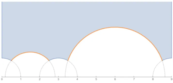
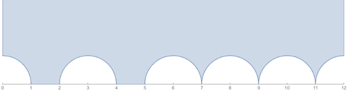
and except for the last chapter even this we will only need forq = 4. If Γ⁰ is a finite index

Figure 1.2: A fundamental domain for Γ₀(4).

subgroup of Γ it acts on P¹(Q) =Q∪ {∞} and has finitely many orbits. These orbits of Γ⁰ are called the cusps of Γ⁰. They are frequently identified with a representative that is in the closure of a fundamental domain inHwhen viewed as a subset of P¹(C). Ifcis a cusp, we let Γ⁰_c be the stabilizer of one of its representatives, (choosing a different representative leads to a Γ⁰ conjugate subgroup). If c =a/c, (a, c) = 1 and γ = [^{a b}_{c d}] ∈Γ, then c =γ∞, and so γ⁻¹Γ⁰_cγ fixes ∞, and as such is a finite index subgroup of Γ∞. We call this index the width of c.

Some simple observations follow [72] . Letc be a cusp of Γ₀(q). Then cis equivalent to some û_v for whichv|q. Moreover û_v, and û_v⁰0 give rise to the same cusp, if and only ifv =v⁰, and u≡u⁰ mod (v, q/v). The width of the cusp û_v is _(v2^q,q).

For example, whenq = 4, there are 3 cusps,∞, 0, and 1/2, of width 1, 4 and 1 see the figure above.

1.8 Half integral weight modular forms

Half integral weight modular forms generalize the (modified) Jacobi theta series, θ(z) = Im(z)^1/4X

n∈Z

e(n²z), which is a modular form of weight 1/2 for Γ₀(4). Set

J(γ, z) = θ(γz)

θ(z) for γ ∈Γ0(4). (1.8.1)

(16)

Say F defined on H has weight 1/2 for Γ0(4) if

F(γz) = J(γ, z)F(z) for all γ ∈Γ0(4).

There is a parallel (yet more intricate) development for Maass forms of weight 1/2. The invariant Laplace operator of weight 1/2 is given by

∆_1/2 =y²(∂_x²+∂_y²)− ¹₂iy∂_x.

A Maass form of weight 1/2 for Γ₀(4) has weight 1/2, is smooth and satisfies ∆_1/2F + λF = 0, where we write λ=λ(F) = ¹₄ + (^r₂)². Such a form has Fourier expansion

ψ(z) =X

n6=0

b(n)W¹

4signn,^ir₂(4π|n|y)e(nx). (1.8.2) Usually we also require some growth conditions as well in the three cusps of Γ0(4). In particular, a Maass cusp form F is in L²(Γ₀(4)\H, dµ) and has the further property that its zeroth Fourier coefficient in each cusp vanishes.

The resolvent kernel G1/2(z, z⁰;s) for ∆_1/2 in this case was also studied by Fay [48] (see also [106]). It satisfies

∆_1/2+s(1−s) Z

Γ0(4)\H

G¹

2(z, z⁰;s)u(z)dµ(z) = u(z⁰) (1.8.3) for u ∈ L²(Γ₀(4)\H, dµ) with weight 1/2. By Theorem 3.1 of [48] we have the Fourier expansion¹

G1/2(z⁰, z;s) =X

n

F1/2,n(z, s)W¹

4signn,s−¹₂(4π|n|y⁰)e(−nx⁰) valid for Imz⁰ >Imz, where for n 6= 0 and Re(s)>1

F¹/2,n(z, s) = ^Γ(s−

1 4signn) 4π|n|Γ(2s)

X

γ∈Γ∞\Γ0(4)

J(γ, z)⁻¹f¹/2,n(γz, s) (1.8.4) with

f1/2,n(z, s) = M¹

4signn,s−¹

2(4π|n|Imz)e(nRez).

As in the weight 0 case, we have the following

Proposition 1.8.1. F1/2,n(z, s) has a meromorphic continuation toRe(s)>0 with simple poles at the points ¹₂ +^ir₂ giving the discrete spectrum of ∆_1/2 and that

Res_s=¹

2+^ir₂(2s−1)G_1/2(z⁰, z) =X

ψ(z⁰)ψ(z) and

Res_s=¹

2+^ir₂(2s−1)F1/2,n(z, s) = X

ψ

b(n)ψ(z). (1.8.5)

Here the sum is over an orthonormal basis {ψ} of Maass cusp forms for V_r andb(n) is as 1.8.2.

1Note that in the notation of Fay,F1/2,n(z, s) =−Fn(z, s). The minus sign comes from his definition of

∆_1/2.We are also using his (38), which givesG1/2(z, z⁰;s) =G1/2(z⁰, z;s).Observe as well that for weight 1/2 hisk= 1/4.

(17)

1.9 Hecke operators and Shimura-Shintani correspon- dence

In this section we denote by U the space of cusp forms of weight 0 and U_r the space of cusp forms of eigenvalue 1/4 +r². Similarly V is the space of weight 1/2 cusp forms, and V_r those cusp forms with spectral parameter 1/2 +ir/2.

For each m one also has the Hecke operator T(m) acting on U [72], these operators commute with each other and ∆, therefore preserving U_r. If ϕis also an eigenform of the Hecke operators then one knows that a(1)6= 0, and we may assume thata(1) = 1. We will call such a form Hecke-normalized.

It is known that the space U_r has a basis of Hecke-normalized eigenforms {ϕ}.

Furthermore we can also assume that a(−n) = a(−1)a(n) = ±a(n). If a(−1) = 1 we say thatϕis even, otherwise odd sinceϕ(−z) = a(−1)ϕ(z). Thus the associatedL-function has an Euler product (for Re(s)>1):

L(s;ϕ) =X

n≥1

a(n)n^−s= Y

pprime

(1−a(p)p^−s+p^−2s)⁻¹. (1.9.1)

The space V is equipped with Hecke operators T_1/2(m²) [118]. There is an important distinguished subspace of V_r, denoted by V_r⁺ and called after Kohnen [82] the plus space, that contains those Maass cusp forms ψ ∈ V_r whose n-th Fourier coefficient b(n) vanishes unless n≡0,1 mod 4. It is clearly invariant under ∆_1/2.

It is shown in [77] that V_r⁺ has an orthonormal basisB_r ={ψ}consisting of eigenfunction of all Hecke operators T_1/2(p²) wherep > 2 is prime. Fix such a basisB_r.

Given ψ ∈B_r with Fourier expansion ψ(z) =X

n6=0

b(n)W¹

4signn,^ir₂(4π|n|y)e(nx) (1.9.2) and a fundamental discriminant d with b(d) 6= 0 the Hecke relation T_1/2(p²)ψ = a_ψ(p)ψ implies that

L_d(s+ ¹₂)X

n≥1

b(dn²)n^−s+1 =b(d)Y

p

(1−a_ψ(p)p^−s+p^−2s)⁻¹. Define the numbersa_ψ(n) via

Y

p

(1−a_ψ(p)p^−s+p^−2s)⁻¹ =X

n≥1

a_ψ(n)n^−s (1.9.3)

and let

Shimψ(z) =y^1/2X

n6=0

2a_ψ(|n|)K_ir(2π|n|y)e(nx). (1.9.4) Note that for some d we must have that b(d)6= 0 so that this is always defined.

Theorem 1.9.1 (Shimura lift). If ψ ∈ Vr is an eigenfunction of all 1/2-weight Hecke operators, then Shimψ ∈U_r and is also an eigenform of all weight 0 Hecke operators.

(18)

1.10 Holomorphic modular forms and functions

Let Γ⁰ ≤ Γ BE a subgroup of finite index, and let f : H → C be a holomorphic function that satisfies

f

az+b cz+d

= (cz+d)^kf(z) (1.10.1)

whenever [^{a b}_{c d}] ∈Γ⁰. Such a form is called weakly holomorphic. We will now assume that Γ⁰ = Γ. In particular we have T ∈Γ⁰ and so we have

f(z+ 1) =f(z).

It follows from this that there is ˜f :{0<|q|<1} →C, holomorphic such that

f(z) = ˜f(e^2πiz) (1.10.2)

We will say f is holomorphic (resp. meromorphic) at ∞ if ˜f is holomorphic (resp.

meromorphic) at 0. For ease of notation we will denote

q=e^2πiz (1.10.3)

so that by (1.10.2) we have

f(z) =X

n

a_nqⁿ (1.10.4)

for some a_n ∈C, called the Fourier coefficients of f.

Definition 1.10.1. We let

M_k^! ={f :H →C:f satisfies 1.10.1, f(z) =

∞

X

n=n0

anqⁿ, for some n0} Similarly let

M_k ={f :H →C:f satisfies 1.10.1, f(z) =

∞

X

n=0

a_nqⁿ} and

S_k ={f :H →C:f satisfies 1.10.1, f(z) =

∞

X

n=1

a_nqⁿ} For example let

E₄(z) = 1 + 240

∞

X

n=1

n³qⁿ 1−qⁿ E6(z) = 1−504

∞

X

n=1

n⁵qⁿ 1−qⁿ and

∆(z) = 1

1728 E₄³(z)−E₆²(z) .

Then E₄ ∈ M₄, E₆ ∈ M₆ and ∆ ∈ S₁₂. Moreover ∆ does not vanish on H and the function

j(z) = E₄³(z)

∆(z)

is invariant. Clearly it is in M₀^!, the space of meromorphic modular functions, and it is well known classically that M₀^! = C(j). The map j : H → C is conformal except at the orbits of i and −¹₂ +

√3

2 i. It establishes a bijection between Γ\H and C.

(19)

1.11 Closed geodesics

There are three closely related ways to describe closed geodesics. All three will appear in the thesis.

Hyperbolic elements

Letσbe hyperbolic, with fixed pointsw1, w2. The geodesicSσconnecting the two endpoints becomes a closed geodesic in Γ\H. This requires some clarifying because Γ\H is only an orbifold. Since σ is hyperbolic, it has real eigenvalues say λ₁ > λ₂, which we may assume are positive after replacing σ by −σ if necessary. Then we have

σ

w₁ w₂

1 1

=

w₁ w₂

1 1

λ₁ 0 0 λ₂

and we can define

σ(t) =

w₁ w₂

1 1

λ^t₁ 0 0 λ^t₂

w₁ w₂

1 1

⁻¹ .

If we now fix a point z₀ on S_σ, then the image of the (parametrized) curve t →σ(t)z₀ becomes periodic on Γ\H with period 1. This may not be the minimal period, if it is we call σ primitive. Then σ is primitive if and only if it is not a positive power of another hyperbolic element. Since the eigenvalues λ₁, λ₂ are units in the maximal order O of K_σ =Q(p

(a+d)²−4), σis primitive if and only if the eigenvalues are the totally positive fundamental unitsD >1/D, whereDis the discriminant ofO. The above parametrization is not by arc-length, the length of a primitive closed geodesic is easy to compute and is

length(C_A) = 2 log_D. (1.11.1)

where _D is the totally positive fundamental unit in O.

It is easy to see that conjugate hyperbolic elements give the same curve in Γ\H.

Real quadratic extensions

Let K/Q be a real quadratic field. Then K=Q(√

D) where D >1 is the discriminant of K. Letw7→w⁰ be the non-trivial Galois automorphism ofKand forα∈KletN(α) =αα⁰. Let Cl⁺(K) be the group of fractional ideal classes taken in the narrow sense. Thus two ideals a and b are in the same narrow class if there is a α ∈ K with N(α) > 0 so that a= (α)b. Let h(D) = #Cl⁺(K) be the (narrow) class number and_D >1 be the smallest unit with positive norm in the ring of integersO_K ofK. We denote byI the principal class and by J the class of the different (√

D) of K, which coincides with the class of principal ideals (α) whereN(α) = αα⁰ <0. Then

Cl(K) = Cl⁺(K)/J

is the class group in the wide sense. Clearly J 6= I iff O_K contains no unit of norm −1.

In this case each wide ideal class is the union of two narrow classes, say A and J A. A sufficient condition for J 6=I is thatD is divisible by a prime p≡3 (mod 4).

For a fixed narrow ideal class A ∈ Cl⁺(K) and a = wZ+Z ∈ A with w > w⁰ let S_w be the geodesic in H with endpoints w⁰ and w. The modular closed geodesic C_A on Γ\H

(20)

is defined as follows. Define γw =±[^{a b}_{c d}]∈Γ, where a, b, c, d∈Zare determined by

_Dw=aw+b (1.11.2)

_D =cw+d,

with _D our unit. Then γ_w is a primitive hyperbolic transformation in Γ with fixed points w⁰ and w. Since

(cw+d)⁻² =⁻²_D <1,

we have that w is the attracting fixed point of γ_w. This induces on the geodesic S_w a clock-wise orientation. Distinct a and w for A induce Γ-conjugate transformations γ_w. If we choose some pointz₀ onS_wthen the directed arc onS_w fromz₀toγ_w(z₀), when reduced modulo Γ, is the associated closed geodesic C_A on Γ\H. It is well-defined for the class A and gives rise to a unique set of oriented arcs (that could overlap) in F. We also use C_A to denote this set of arcs. Again it is well-known and easy to see using (1.11.2) that

length(C_A) = 2 log_D. (1.11.3)

Binary quadratic forms

In place of ideal classes, it is sometimes more convenient to use binary quadratic forms Q(x, y) = [a, b, c] =ax²+bxy+cy²,

wherea, b, c∈ZandD=b²−4ac.Quadratic forms are especially useful when one wants to consider arbitrary discriminants D. For fundamental D all quadratic forms are primitive in that gcd(a, b, c) = 1 and we have a simple correspondence between narrow ideal classes of K and equivalence classes of binary quadratic forms of discriminant D with respect to the usual action of PSL(2,Z). This correspondence is induced by a 7→ Q(x, y), where a=wZ+Z with w^σ < w and

Q(x, y) =N(x−wy)/N(a).

The map takes the narrow ideal class ofato the Γ-equivalence class ofQ. The inverse map is given by Q(x, y)7→wZ+Z where

w= −b+√ D 2a ,

provided we chooseQ in its class to havea >0. The following table of correspondences is useful. Suppose that Q= [a, b, c] represents in this way the ideal class A. Then

[a,−b, c] represents A⁻¹ (1.11.4)

[−a, b,−c] represents J A (1.11.5)

[−a,−b,−c] represents J A⁻¹. (1.11.6) For a primitive quadratic form Q(x, y) = [a⁰, b⁰, c⁰] with any non-square discriminant d⁰ >1 its group of automorphs in Γ is generated by

γ_Q=± _t−b0u

2 −c⁰u a⁰u ^t+b₂⁰^u

, (1.11.7)

(21)

where (t, u) gives the smallest integer solution with t, u≥1 to t²−d⁰u² = 4

(see [108]).

If

Q(x, y) = N(x−wy)/N(a) as above then γ_Q = γ_w and ε_D = ^t+u

√ D

2 . Therefore the closed geodesic associated to the hyperbolic element γ_Q agrees with the closed geodesic associated to the narrow class A.

Using (1.11.6) we see that the closed geodesicC_{J A}⁻¹ has the same image asC_Abut with the opposite orientation.

It is also possible to describe the primitive quadratic form associated to a hyperbolic element. If σ = ^{a b}_{c d}

is a primitive hyperbolic element, then let u = gcd(c, d−a, b) and set

Q_σ(z) =−c

uX²+a−d

u XY + b uY²,

then Q_σ is primitive and its group of automorphs is generated by σ_Q_σ =σ.

When D > 0 and Q is primitive and n ∈ Z⁺ define C_nQ = C_Q. When D < 0 let zQ = ^−b+

√ D

2a ∈ H if Q= [a, b, c] and let ωQ be the number of automorphs of Qin Γ.

Remark 1.11.1. The arcs of C_A might retrace back over themselves. When this happens C_A is said to bereciprocal. In terms of the classA, it means thatJ A⁻¹ =Aor equivalently A² =J. Sarnak [110] has given a comprehensive treatment of these remarkable geodesics for arbitrary discriminants.

1.12 Genus characters

We need to define genus characters for arbitrary discriminants. We will mainly use the language of binary quadratic forms. Let Q_D be the set of Q with discriminant D that are positive definite when D < 0. For Q = [a, b, c] with discriminant D = d⁰d where d is fundamental we define

χ(Q) = ( d

m

if (a, b, c, d) = 1 where Qrepresents m and (m, d) = 1, 0, if (a, b, c, d)>1.

Now assume that d is a fundamental discriminant and that D = dd⁰. We need an associated exponential sum, defined for c≡0 (mod 4) by

S_m(d⁰, d;c) = X

b(modc) b²≡D(modc)

χ [₄^c, b,^b²^−D_c ]

e ^2mb_c

. (1.12.1)

Clearly

S−m(d⁰, d;c) = S_m(d⁰, d;c) = S_m(d⁰, d;c).

We have the identity

χ_d(−Q) = (sgnd)χ_d(Q). (1.12.2)

(22)

A crucial ingredient in what follows is an identity connecting the weight 1/2 Klooster- man sum withS_m(d, d⁰;c) above. In a special case this identity is due to Sali´e and variants have found many applications in the theory of modular forms. We shall use a general version due essentially to Kohnen [83]. To define the weight 1/2 Kloosterman sum we need an explicit formula for the theta multiplier in J(γ, z) =θ(γz)/θ(z) introduced above.

This may be found in [118, p. 447]. As usual, for non-zero z ∈ C and v ∈ R we define z^v =|z|^vexp(ivargz) with argz ∈(−π, π]. We have

J(γ, z) = (cz+a)^1/2ε⁻¹_a _a^c

for γ =±[^{∗ ∗}_{c a}]∈Γ₀(4), where ^c_a

is the extended Kronecker symbol and ε_a =

(1 if a≡1 (mod 4) i if a≡3 (mod 4).

For c∈Z⁺ with c≡0 (mod 4) and m, n∈Z let K_1/2(m, n;c) = X

a(modc) c a

ε_ae ^ma+na_c

be the weight 1/2 Kloosterman sum. Here a ∈Zsatisfies aa≡1 (mod c).

It is convenient to define the modified Kloosterman sum K⁺(m, n;c) = (1−i)K_1/2(m, n;c)×

(1 if c/4 is even

2 otherwise. (1.12.3)

It is easily checked that

K⁺(m, n;c) =K⁺(n, m;c) =K⁺(n, m;c). (1.12.4) The following identity is proved by a slight modification of the proof given by Kohnen in [83, Prop. 5, p. 259] (see also [35], [75] and [124]).

Proposition 1.12.1. For positive c≡0 (mod 4), d, m∈ Z with d ≡0,1 (mod 4) and D a fundamental discriminant, we have

S_m(d, D;c) = X

n|(^m,₄^c)

D n

q

n c K⁺

d,^m_n²2^D;_n^c .

By M¨obius inversion in two variables this can be written in the form c^−1/2K⁺(d, m²D, c) = X

n|(^m,^c4)

µ(n) ^D_n

S_m/n d, D;_n^c

. (1.12.5)

Note that this gives an identity for K⁺(d, d⁰, c) for any pair d, d⁰ ≡ 0,1 (mod 4). An immediate consequence of (1.12.5) and the obvious upper bound

S_m(d, D;c) c

(23)

is the upper bound

K⁺(d, d⁰, c) c^1/2+, (1.12.6) which holds for any >0.Furthermore, since for any m, n∈Zwe have

K_1/2(m, n;c) = ¹₄K_1/2(4m,4n; 4c), (1.12.6) implies that for any m, n∈Z

K_1/2(m, n, c)c^1/2+.

This elementary bound correspond to Weil’s bound for the ordinary (weight 0) Kloosterman sum

K₀(m, n;c) = X

a(modc) (a,c)=1

e ^ma+na_c ,

which states that (see [128], [66, Lemma 2])

K₀(m, n;c) (m, n, c)^1/2c^1/2+. (1.12.7)

(24)

Chapter 2 The Shimura-Shintani

correspondence and formulas of Katok-Sarnak type

2.1 Background and statements of results

Correspondences between automorphic forms on different groups have a long and rich history as can be seen in the works of Doi-Naganuma, Shimura, Langlands and many others. The Shimura-Shintani [118, 119] correspondence lead to many applications via the formulas of Waldspurger [125] and Kohnen-Zagier [84]. The analogous formula in case of Maass forms was given by Katok and Sarnak[77]. A particularly important application of such formulas is due to Duke on the equidistribution of CM points and closed geodesics [35]. There are various methods for proving this family of formulas that use either theta- kernels, or spectral methods [11]. Recently an extension of the Katok-Sarnak formula was developed in [41] with applications to a new type of equidistribution result. In this chapter we will present the part of the paper where this extension is proved.

2.1.1 Katok-Sarnak type formulas

Let u(z) = E(z, s),. We recall a version of a classical formula of Hecke. Let L(s, χ_d) be the DirichletL-function with character given by the Kronecker symbolχ_d(·) = ^d_·

and for α= ¹₂(1−signd) define the completedL-function

Λ(s, χ_d) = π^−s/2Γ(^s+a₂ )|d|^s/2L(s, χ_d). (2.1.1) Theorem 2.1.1. For the genus characterχ associated to D=d⁰d and Re(s) = ¹₂ we have

Λ(s, χ_d⁰)Λ(s, χ_d) =X

Q∈

χ(Q)





 R

CQi∂_zE^∗(z, s)dz if d⁰, d <0 R

CQE^∗(z, s)y⁻¹|dz| if d⁰, d >0 2√

πω_D⁻¹ E^∗(z_A, s) if d⁰d <0.

This formula is due to Hecke except when d⁰, d <0. Theorem 2.1.1 can be expressed in terms of Maass forms of weight 1/2.

Set for fundamental d

b(d, s) = (4π)^−1/4|d|^−3/4Λ(s, χ_d)

(25)

and define b(dm², s) form ∈Z⁺ by means of the Shimura relation

mX

n|m n>0

n⁻³² ^d_n

b ^m_n²2^d, s

=m^s−1/2σ1−2s(m)b(d, s).

Then it follows from [40, Proposition 2 p.959] that E_1/2^∗ (z, s) = Λ(2s)2^sy²^s⁺¹⁴ + Λ(2−2s)2^1−sy³⁴⁻^s²+

X

n≡0,1(mod 4) n6=0

b(n, s)W¹

4sgnn,^s₂−¹₄(4π|n|y)e(nx) has weight 1/2 for Γ₀(4). The idea behind this example originates in the papers of H.

Cohen [27] and Goldfeld and Hoffstein [51]. See also [117], [34].

The formula

Λ(s, χ_d⁰)Λ(s, χ_d) = 2√

π|D|^3/4b(d⁰, s)b(d, s) (2.1.2) in connection with Theorem 2.1.1 hints strongly as to what should take place for cusp forms; this is the extension (and refinement) of the formula of Katok-Sarnak mentioned earlier. Their result from [77], together with [8], gives the case d= 1 in the following.¹ Theorem 2.1.2 ([43]). Let

ϕ(z) = 2y^1/2X

n6=0

a(n)Kir(2π|n|y)e(nx)

be a fixed even Hecke-Maass cusp form for Γ. Then there exists a unique nonzero F(z) with weight 1/2 for Γ₀(4) with Fourier expansion

F(z) = X

n≡0,1(mod 4) n6=0

b(n)W¹

4sgnn,^ir₂(4π|n|y)e(nx),

such that for any pair of co-prime fundamental discriminants d⁰ and d we have

12√

π|D|³⁴ b(d⁰)b(d) =hϕ, ϕi⁻¹X

Q∈

χ(Q)





 R

CQi∂zϕ(z)z if d⁰, d <0 R

CQϕ(z)y⁻¹|dz| if d⁰, d >0 2√

π ω⁻¹_D ϕ(z_Q) if d⁰d <0,

(2.1.3)

where χ is the genus character associated to D = d⁰d. Here hF, Fi = R

Γ0(4)\H|F|²dµ = 1 and the value of b(n) for a general discriminant n = dm² for m ∈ Z⁺ is determined by means of the Shimura relation

mX

n|m n>0

n⁻³² _n^d b ^m_n²2^d

=a(m)b(d).

1Except that whend⁰<0 we get in (2.1.3) on the RHS 2√

π ω⁻¹_D instead of their (2√

π ω_D)⁻¹.

(26)

Remarks. The √

π in (2.1.2) and (2.1.3) is an artifact of the normalization of the Whit- taker function. Also, if we choose F in Theorem 2.1.2 so that hF, Fi = 6, which is the index of Γ₀(4) in Γ, then we get 2 in the LHS of (2.1.3) instead of 12, which matches the Eisenstein series case (2.1.2). Perhaps not coincidentally,

Res_s=1E_1/2^∗ (z, s) = ¹₂θ(z) and by [26] we have h¹₂θ(z),¹₂θ(z)i= 6.

It is also possible to evaluate |b(d)|². When d= 1 this was done in [77] and in general by Baruch and Mao [8]. Here we quote their result in our context. Under the same assumptions as in Theorem 2.1.2 we have

12π|d||b(d)|² =hϕ, ϕi⁻¹Γ(¹₂ +^ir₂ −^sign₄ ^d)Γ(¹₂ − ^ir₂ − ^sign₄ ^d)L(¹₂, ϕ, χ_d), (2.1.4) where

L(s, ϕ, χ_d) = X

n≥1

χ_d(n)a(n)n^−s.

Hence in the cuspidal case our problem also reduces to obtaining a sub-convexity bound, this time for a twisted L-function.

Results like Theorem 2.1.2 and (2.1.4) have a long history, especially in the holomorphic case. Some important early papers are those by Kohnen and Zagier [84], Shintani [119]

and Waldspurger [125]. All of these relied on the fundamental paper of Shimura [118].

Examples

It is interesting to evaluate numerically some examples of Theorem 2.1.2. This is possible thanks to computations done by Str¨omberg [122]. Note that half-integral weight Fourier coefficients, even in the holomorphic case, are notoriously difficult to compute.

For example, forϕ(z) we take the first occurring even Hecke-Maass form with eigenvalue λ= 190.13154731· · ·= ¹₂ +r²,

where r/2 = 6.889875675. . . . We have

hϕ, ϕi= 7.26300636×10⁻¹⁹.

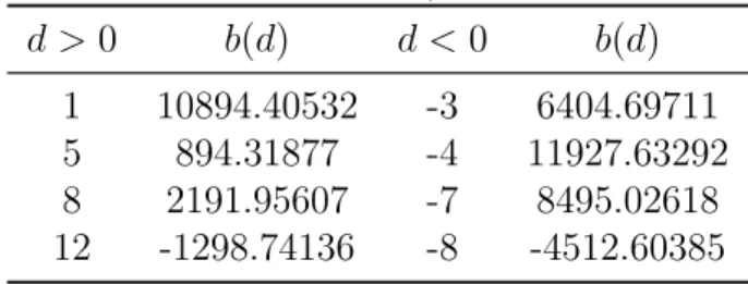
A large number of Hecke eigenvalues for this ϕ are given (approximately, but with great accuracy) in the accompanying files of the paper of Booker, Str¨ombergsson and Venkatesh [14]. The first six values to twelve places are given in Table 2.1.

A few values of b(d) for fundamentald (except ford= 1, which we computed indepen- dently) are computed from Str¨omberg’s Table 5 and given in our Table 2.2.

Let us illustrate Theorem 2.1.2 in a few cases. Consider first the quadratic field Q(√ 3), for which D = 12 = 4·3. There are 2 classes: the principal class I with associated cycle ((4)) and J with cycle ((2,3)). For D= 12 = (1)(12)

12^7/4√

π b(1)b(12) = 2hϕ, ϕi⁻¹ Z

∂F_I

ϕ(z)y⁻¹|dz|=−1.94029×10⁹ and for D= (−3)(−4)

12^7/4√

π b(−3)b(−4) =λhϕ, ϕi⁻¹ Z

F_I

ϕ(z)dµ(z) = 1.04759×10¹⁰.

CYCLE INTEGRALS OF MODULAR FORMS DISSERTATION submitted for the degree of “Doctor of the Hungarian Academy of Sciences” Árpád Tóth Eötvös Loránd University