RESEARCH ARTICLE
Extended similarity indices:
the benefits of comparing more than two objects simultaneously. Part 1: Theory
and characteristics †
Ramón Alain Miranda‑Quintana1* , Dávid Bajusz2 , Anita Rácz3 and Károly Héberger3*
Abstract
Quantification of the similarity of objects is a key concept in many areas of computational science. This includes cheminformatics, where molecular similarity is usually quantified based on binary fingerprints. While there is a wide selection of available molecular representations and similarity metrics, there were no previous efforts to extend the computational framework of similarity calculations to the simultaneous comparison of more than two objects (mol‑
ecules) at the same time. The present study bridges this gap, by introducing a straightforward computational frame‑
work for comparing multiple objects at the same time and providing extended formulas for as many similarity metrics as possible. In the binary case (i.e. when comparing two molecules pairwise) these are naturally reduced to their well‑
known formulas. We provide a detailed analysis on the effects of various parameters on the similarity values calculated by the extended formulas. The extended similarity indices are entirely general and do not depend on the fingerprints used. Two types of variance analysis (ANOVA) help to understand the main features of the indices: (i) ANOVA of mean similarity indices; (ii) ANOVA of sum of ranking differences (SRD). Practical aspects and applications of the extended similarity indices are detailed in the accompanying paper: Miranda‑Quintana et al. J Cheminform. 2021. https:// doi.
org/ 10. 1186/ s13321‑ 021‑ 00504‑4. Python code for calculating the extended similarity metrics is freely available at:
https:// github. com/ ramir andaq/ Multi pleCo mpari sons.
Keywords: Comparisons, Rankings, Extended similarity indices, Consistency, Molecular fingerprints, ANOVA, Sum of ranking differences
© The Author(s) 2021. This article is licensed under a Creative Commons Attribution 4.0 International License, which permits use, sharing, adaptation, distribution and reproduction in any medium or format, as long as you give appropriate credit to the original author(s) and the source, provide a link to the Creative Commons licence, and indicate if changes were made. The images or other third party material in this article are included in the article’s Creative Commons licence, unless indicated otherwise in a credit line to the material. If material is not included in the article’s Creative Commons licence and your intended use is not permitted by statutory regulation or exceeds the permitted use, you will need to obtain permission directly from the copyright holder. To view a copy of this licence, visit http:// creat iveco mmons. org/ licen ses/ by/4. 0/. The Creative Commons Public Domain Dedication waiver (http:// creat iveco mmons. org/ publi cdoma in/
zero/1. 0/) applies to the data made available in this article, unless otherwise stated in a credit line to the data.
Introduction
A large number of molecular representations exist, and there are several methods (similarity and dis- tance measures) to quantify the similarity of molecular
representations [1, 2]. These similarity and distance measures (coefficients) accompany the entire process of drug design: virtual screening, [3] hit-to-lead optimiza- tion, [4] QSAR modeling, [5] finding activity cliffs, [6]
drug target prediction, [7] etc.
Molecular similarity has been established as the basis of ligand-based virtual screening, as well as molecular informatics (a collective term encompassing various spe- cific applications of cheminformatics principles, such as compound library design or molecular property predic- tions) [8]. Information theory has also provided some metrics on similarity. However, molecular similarity plays
Open Access
*Correspondence: quintana@chem.ufl.edu; heberger.karoly@ttk.hu
1 Department of Chemistry, University of Florida, Gainesville, FL 32603, USA3 Plasma Chemistry Research Group, ELKH Research Centre for Natural Sciences, Magyar tudósok krt. 2, 1117 Budapest, Hungary
Full list of author information is available at the end of the article . † Part 2 is available at: https:// doi. org/ 10. 1186/ s13321‑ 021‑ 00504‑4
a crucial role in quantum chemistry as well [9–14]. The merits of pairwise fingerprint comparisons have been exhausted on a large scale [15]. Todeschini et al. summa- rized many of the binary similarity coefficients that have been developed so far [1, 16].
In our earlier works we have investigated the appli- cability of binary similarity coefficients, proved their equivalency or superiority [17–19]. We could find better similarity coefficents than the most frequently applied Tanimoto index [2] and formulated constraints about finding the best equations for fitting data [20].
It is somewhat odd that the similarity evaluations are exclusively based on pairwise comparisons of two mol- ecules. By analogy, multiple linear regression is not exclu- sively based on univariate correlations between each predictor and the response, but takes into account multi- ple correlations. (Two descriptors together might be sig- nificant in a model predicting the response whereas none of them correlates with it significantly alone.) Hence, it is natural to consider the extension of the standard com- parative indices such that they can be used to compare more than two objects (e.g., molecules, fingerprints) at a time. This will provide unparalleled flexibility to the tra- ditional algorithms that aim to quantify molecular simi- larity, since one will have the freedom of choosing how many molecules are to be compared simultaneously. This will in turn allow us to gain further insight regarding the relations among the compounds in a given dataset (by providing more complete measures of chemical diver- sity), which can then be used to shed more light on their structures and properties.
While to our knowledge, comparing multiple objects at the same time has not yet been introduced for molecu- lar fingerprints, it is worth to note that other studies have combined multiple comparative measures in other contexts in the field. For example, in a recent study, an iterative virtual screening strategy was designed and eval- uated on 25 diverse bioactivity data sets from ChEMBL, to benchmark the performance of multiple machine learning methods [7]. The study emulates the typical scenario of early drug discovery (lots of data on inactive compounds vs. almost no information on actives) and extends the comparisons to multitarget drug discovery setups, where activities are predicted simultaneously for more drug targets. Another example is Pareto-Optimal Embedded Modeling (POEM), a non-parametric, super- vised machine learning algorithm developed to generate reliable predictive models without need for optimization.
POEM’s predictive strength is obtained by combining multiple different representations of molecular structures [21].
In this study we propose a novel alternative to pairwise similarity calculations. Instead of using multiple binary
comparisons to analyze a dataset, we present multiple classes of comparative measures that can be used to com- pare an arbitrary number of molecules at the same time.
The central element of our work is to provide a general framework for comparing multiple objects at the same time, which naturally extends the range of validity of most of the similarity indices commonly used in chemin- formatics and drug design. This was based on a compre- hensive analysis of the binary similarity measures defined so far, which allowed us to identify their fundamental defining features (e.g., similarity/dissimilarity counters, coincidence thresholds), which are the key to defin- ing fully general n-ary similarity indices. We performed variance analyses in order to decompose the effects of various factors: number of molecules compared simul- taneously, effect of weighting, types of similarity coeffi- cients, and length of the fingerprint. These new families of indices considerably expand the scope of the com- parative analysis since they provide new dimensions to what is currently achievable with standard binary com- parisons. Moreover, beyond their intrinsic theoretical interest, we anticipate that n-ary comparisons can have important practical applications ranging from estimat- ing set-similarity to providing new rigorous ways to study chemical diversity and explore compound databases. In particular, we have found that calculating the introduced n-ary comparisons for large datasets is excessively faster than the traditional approach of calculating full pairwise similarity matrices to quantify the diversity of a com- pound set. After introducing the theoretical basis of the n-ary fingerprint comparisons here, we share our detailed results on the practical applicability of this framework in the accompanying paper [(part 2) 22]. Meanwhile, the Python code for calculating the extended similarity met- rics is freely available at https:// github. com/ ramir andaq/
Multi pleCo mpari sons.
Theory of fingerprint comparisons Binary comparisons
Similarity measures/indices are generally presented as binary relations, in the sense that they assign a (real) number to a pair of molecules. These relations are based on a suitable representation of the molecules, either in terms of graphs, lexicographical tools (like the SMARTS or SMILES formats), field-based quantities (like the electron density or the molecular electrostatic poten- tial), or the widely used molecular fingerprints. Here, we will focus on the latter, particularly on the well-known binary fingerprints, where a molecule is represented as a string of 1′s and 0′s (without restricting the scope of our approach).
It is important to point out that the word “binary” has two meanings in our context. On the level of fingerprints,
it means that a fingerprint consists of a string of two pos- sible values (0 and 1). Let us call such strings as dichoto- mous variables further on. On the level of comparisons, it means that two objects (molecules, fingerprints) are compared simultaneously. Since in the present work, we exclusively apply binary (dichotomous) fingerprints, our use of the word “binary” will refer to comparisons of two objects/molecules, in contrast to the simultaneous com- parison of multiple objects (“n-ary comparisons”), which is the central concept of this study.
In the case of the binary comparison of (dichotomous) fingerprints, there are four basic quantities that we can calculate for each pair of fingerprints:
a: the number of coincident 1′s (number of common on bits).
b: number of 1′s present in the first fingerprint but absent in the second.
c: number of 1′s present in the second fingerprint but absent in the first.
d: the number of coincident 0′s (number of common off bits).
For instance, in the following example:
a = 2, b = 2, c = 1, d = 3.
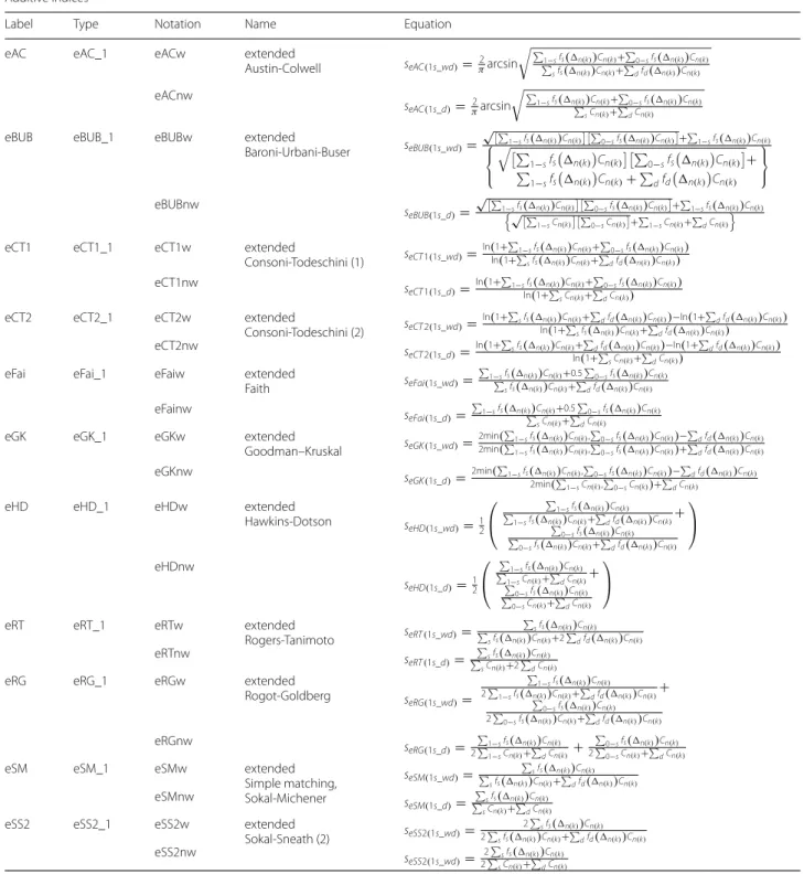
These numbers can then be combined in many differ- ent ways in order to define multiple similarity indices (for a comprehensive list see the Additional file 1). In general, the similarity indices have the following form:
where Gi, gi1 and gi2 represent functions in general. For example, the Kulczynski (Kul) index is given by:
Nonetheless, there are other indices (which we will call additive) for which we only need the sum of b and c, namely:
like the Sokal-Michener (SM) index:
where p = a + b + c + d.
A=(10110100) (1) B=(00100101)
(2) s=
iGi
gi1(a,d,b,c) gi2(a,d,b,c)
(3) sKul = 1
2
a
a+b+ a a+c
(4) s=
iGi
gi1(a,d,b+c) gi2(a,d,b+c)
(5) sSM = a+d
p
Finally, within the additive indices we encounter a sub- class of indices that we will call asymmetric, because they depend on a, but not on d, that is:
a representative example of this class would be the Jac- card-Tanimoto (JT) index (widely known as Tanimoto similarity in the cheminformatics and drug discovery communities):
n‑ary comparisons
In the effort to extend the expressions of the binary com- parisons in order to simultaneously compare an arbitrary number n of molecular fingerprints (n-ary comparisons), the first step is to introduce the notation Cn(k) to repre- sent the number of times that we find k coinciding 1′s between n bitstrings (irrespective of the order in which we consider the fingerprints). (Notice that 0≤k≤n .) For instance, in the binary (n = 2) case: C2(2)=a , C2(1)=b+c , C2(0)=d . Obviously, with this simple notation we can only discuss additive indices for now (see Eq. 4). We defer to a future work a discussion of n-ary comparisons applicable to general indices Eq. (2).
The key detail that we need to notice is that, in the case of binary comparisons, pairs of fingerprints with large values of a and d will be more similar, and pairs of fin- gerprints with large values of b and c will be less simi- lar. Then, it makes sense to classify a and d as similarity counters (in particular, a will be a 1-similarity counter and d a 0-similarity counter), and b and c as dissimilar- ity counters. Extending this notion to n-ary comparisons requires us to classify Cn(k) as similarity and dissimilarity counters as well. We do this with the help of the follow- ing indicator:
It is clear that a bigger value of �n(k) will imply that the given strings have more elements in common (either 1′s or 0′s). Now we must define a minimum value that determines from what point a given number of occur- rences can be considered as coincident. We will denote this coincidence threshold as γ. There are many possible ways to define this threshold, for instance, a somehow contrived possibility would be to set γ =n
2
(where ⌈x⌉
is the ceiling function). However, perhaps a better option (in the sense that it maximizes the number of similarity counters) will be to take γ =nmod2 . (Roughly speak- ing, this choice of γ means that the fingerprints will be
(6) s=
iGi
gi1(a,b+c) gi2(a,b+c)
(7) sJT = a
a+b+c
(8)
�n(k)= |2k−n|
“similar” at a given position if more than half of the bits have the same value in that position.) In any case, we will take Cn(k) as a similarity counter if �n(k)> γ , and as a dissimilarity counter when �n(k)≤γ . In particular, Cn(k)
will be a 1-similarity counter if 2k−n> γ , and a 0-simi- larity counter if n−2k> γ . Notice that, as expected for the n = 2 case, C2(2) and C2(0) will be 1- and 0-similarity counters, respectively, while C2(1) will be a dissimilarity counter.
Finally, we should discuss the relative relevance that dis- tinct types of similarity and dissimilarity counters have within a given similarity index. For instance, let us consider n = 4 and set γ =0 . In this case, both C4(4) and C4(3) will be 1-similarity counters, but the first one indicates when we
have a 100% coincidence among the compared fingerprints, while the latter indicates when we have a 75% concord- ance among the compared fingerprints. Therefore, it seems natural to weight these counters differently. We can do this according to the following convention: If Cn(k) is a similarity counter, then it should be multiplied by a factor fs
�n(k) that is an increasing function of �n(k) . Contrary, if Cn(k) is
At this point we have all the necessary ingredients to generalize the binary comparisons. An additive index like the one presented in Eq. (4) can now be rewritten as:
Let us briefly explain the notation in the previous expression: the summations over 1-s, 0-s, and d represent the sum over the 1-similarity, 0-similarity, and dissimilar- ity counters, respectively. The subscript 1s_wd indicates that we are distinguishing between the 1- and 0-similar- ity counters (hence the “1” in the similarity “s” part), and that the counters in the denominator are weighted (hence the “w” in the denominator “d” part). We introduce this distinction because we can propose yet another generali- zation for the additive indices, in the form of:
Notice that now we are not weighting the counters in the denominator (which is reflected in the subscript 1s_d).
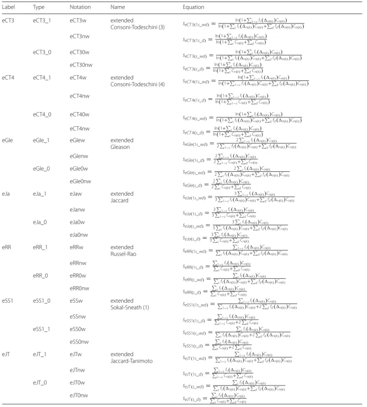
As an example of these two possible extensions, let us once again revisit the SM index (detailed expressions for the remaining additive indices are given in Appendix 1:
Table 1):
Here and in the following we will distinguish the extended (n-ary) versions of the similarity indices by including an “e” as a subscript (notice the difference with respect to Eq. (5).
Since the asymmetric indices are a sub-class of the additive indices they can also be extended in this form, namely:
(10) s1s_wd=
iGi
gi1
1−sfs
�n(k)
Cn(k),
0−sfs
�n(k)
Cn(k),
dfd
�n(k) Cn(k) gi2
1−sfs
�n(k)
Cn(k),
0−sfs
�n(k)
Cn(k),
dfd
�n(k) Cn(k)
(11) s1s_d=
iGi
gi1
1−sfs
�n(k)
Cn(k),
0−sfs
�n(k)
Cn(k),
dfd
�n(k) Cn(k) gi2
1−sCn(k),
0−sCn(k),
dCn(k)
(12) seSM(1s_wd)=
1−sfs
�n(k)
Cn(k)+
0−sfs
�n(k) Cn(k)
1−sfs
�n(k)
Cn(k)+
0−sfs
�n(k)
Cn(k)+
dfd
�n(k) Cn(k)
(13) seSM(1s_d)=
1−sfs
�n(k)
Cn(k)+
0−sfs
�n(k) Cn(k)
1−sCn(k)+
0−sCn(k)+
dCn(k)
(14) s1s_wd=
iGi
gi1
1−sfs
�n(k)
Cn(k),
dfd
�n(k) Cn(k) gi2
1−sfs
�n(k)
Cn(k),
dfd
�n(k) Cn(k)
a dissimilarity counter, it should be multiplied by a factor
fd
�n(k)
that is a decreasing function of �n(k) . In both cases we must have: fs(n)=fd(nmod2)=1 . As it was the case for γ , there are many ways of choosing fs and fd. One possibility would be to set fs
�n(k)
=2−(n−�n(k)) and fd
�n(k)
=2−(�n(k)−nmod2) . However, this might put too harsh a penalty on the different counters. For this reason, in the following we will use instead these weight functions:
(9) fs
�n(k)
= �n(k) n ,fd
�n(k)
=1−�n(k)−nmod2 n
Moreover, there are further possibilities, if we replace the sum over the 1-similarity counters with a sum over all the similarity counters:
Now the summation over s indicates the sum over all similarity counters. Also, we do not include the “1” in the subscript because now we are not distinguishing between the 1- and 0-similarity counters. As it was the case in Eqs. (9) and (10) the presence (absence) of the “w” in the subscript indicates that we are (or are not) weighting the counters in the denominator. In Appendix 2 we include a detailed step-by-step calculation of the SM index for 4-ary and 5-ary comparisons.
Notice that when n = 2 this generalization will be equivalent to substituting a by a + d (and leaving p unchanged wherever it appears). This makes easier to realize that this procedure will be redundant in most cases, in the sense that we will just obtain the expression for an already known (additive) index. This is actually the case for six of the seven asymmetric indices considered here; Consoni-Todeschini (3) (CT3), Consoni-Todeschini (4) (CT4), Gleason (Gle), Russell-Rao (RR), Jaccard-Tani- moto (JT), and Sokal-Sneath (1) (SS1):
The Jaccard (Ja) index is the only one that actually leads to a new result:
(15) s1s_d=
iGi
gi1
1−sfs
�n(k)
Cn(k),
dfd
�n(k) Cn(k) gi2
1−sCn(k),
dCn(k)
(16)
ss_wd=
iGi
gi1
sfs
�n(k) Cn(k),
dfd
�n(k) Cn(k) gi2
sfs
�n(k) Cn(k),
dfd
�n(k) Cn(k)
(17)
ss_d=
iGi
gi1
sfs
�n(k) Cn(k),
dfd
�n(k) Cn(k) gi2
sCn(k),
dCn(k)
sCT3= ln(1ln(1++a)p) (18) sCT4= ln(1+a+b+c)ln(1+a)
→sCT1= ln(1+a+d) ln(1+p)
(19) sGle= 2a
2a+b+c →sSS2= 2a+2d p+a+d
sRR= ap (20)
sJT = a+b+ca →sSM= a+d p
(21) sSS1= a
a+2b+2c →sRT = a+d p+b+c
In the general n-ary case, the four possible variants of the Jaccard index are:
It is important to realize that all of these different gen- eralizations will naturally reduce to the standard binary expressions when we substitute n = 2 in the above formulas.
Before concluding this section, it is worth noting that while we have focused on generalizing different similar- ity indices, the concepts introduced above can be used to generalize several dissimilarity indices. In Appendix 3, we briefly touch on this subject, with the particular case of the Hamming distance.
Computational methods
Development of sum of ranking differences (SRD)
The sum of ranking differences (SRD) algorithm was introduced in 2010, [23] showing practical examples and its validation by a permutation test. SRD was first dem- onstrated to solve method-comparison problems in a fast and easy way: the smaller the sum, the better the method (i.e. closer to the gold standard or best consensus). In the beginning, validation was done by running SRD on randomly generated variables in the size of the input data matrix. The obtained histogram shows whether the ranking is comparable with random ranking (e.g. when the original variables overlap with the random variables) [23]. The theoretical SRD distributions were defined for different sample sizes up to 13. The theoretical SRD can be well approximated with a Gaussian distribution, if the (22)
sJa= 3a
3a+b+c →sJa0= 3a+3d
3a+3d+b+c = 3a+3d p+2a+2d
(23)
seJa(1s_wd)= 3
1−sfs
�n(k) Cn(k)
3
1−sfs
�n(k)
Cn(k)+
dfd
�n(k) Cn(k)
(24) seJa(1s_d)= 3
1−sfs
�n(k) Cn(k) 3
1−sCn(k)+
dCn(k)
(25)
seJa(s_wd)= 3
sfs
�n(k) Cn(k)
3
sfs
�n(k)
Cn(k)+
dfd
�n(k)
Cn(k)
(26) seJa(s_d)= 3
1−sfs
�n(k) Cn(k) 3
1−sCn(k)+
dCn(k)
the number of rows (n) in the input matrix exceeds 13 [24]. Later, the SRD algorithm was extended to repeated observations (ties) [25]. Exact theoretical distributions were derived for 4 < n < 9 and a reasonable approxima- tion works for n > 8, using Gaussian distribution fitted on three million n–dimensional random vectors [25]. Cou- pling SRD with variance analysis (ANOVA) provided a unique way of decomposing the effects of different fac- tors influencing the comparions [26, 27].
Recent examinations have unambiguously shown that sum of ranking differences (SRD) realizes a multicriteria optimization [28, 29]. Lourenço and Lebensztajn have illustrated on two practical examples that SRD realizes a consensus of eight different multicriteria decision mak- ing (MCDM) methods [29], whereas any of the individual ones selects various parts of the Pareto front as optimal.
Hence, the individual usage of any MCDM tools is lim- ited; moreover, the selection of weights is a highly subjec- tive and individual process.
Here, we will use the SRD approach to compare the extended similarity metrics with each other and study the effects of the various possible choices (e.g. weighting, value of n).
Description of the SRD procedure
The variables or methods (here, similarity coefficents) to be compared should be arranged in the columns, and the objects (here, objects are the simulated dichotomous fin- gerprints) are arranged in the rows of the input matrix.
The SRD technique needs a gold standard (benchmark or reference) to be defined for ranking. In lack thereof, this reference can be provided by data fusion as summarized by Willett [30] and should be selected according to the nature of the data.
The SRD algorithm consists of three stages:
1. Definition of the reference vector: Selection of a gold standard (benchmark) depending on the features of the dataset. This is straightforward, if there is a clearly defined reference vector (e.g. experimentally determined reference values); in other cases, data fusion from the compared data vectors is recommended. Perhaps the most frequently applied data fusion possibility is the usage of mean values. The basic assumption of their usage is that the random errors cancel each other out.
The systematic errors behave similarly; provided they are numerous (above or around seven sources). Even if a (small) bias remains we are better off by using the most probable value (consensus) instead of any individual one.
In fact, we have shown that the mean values as reference are inherently robust when including/omitting methods that rank the objects highly consistently, or even identi- cally. [19] Of course other data fusion options also exist:
it is “natural” to select the row minima for residuals,
errors or misclassification rates. Similarly, row maximum is a suitable gold standard for the best classification rates, explained variance, etc. Recently, we have extended SRD with an option to compare each method pair-wise and present the results in a heatmap format [31].
As we have remarked before: “If the true (ideal) rank- ing is not known, it is expedient to substitute it with the average of all methods for each object (row average).
This is the key step: the ranking by average values can be accepted as ’’ideal’’, since the errors cancel each other.”
[23] This is precisely the approach we use here.
2. Calculation: Calculation of absolute differences between each rank-transformed individual vector values and the reference (benchmark) column (ranks, with par- tial rankings being used for ties), and sum the absolute differences for each object (compound) together. These values are called SRD values and rank the individual vari- ables (similarity coefficents). SRD values are normalized between 0 and 100 to obtain comparability between vari- ous data sets. The smaller the SRD value, the closer the variable is to the benchmark (consensus). For an easy visual representation of the SRD procedure, we refer the reader to our earlier work (more specifically an anima- tion, supplied as Additional file 3 in ref. [19]). Because the values in the columns cannot always be strictly monoto- nously ordered, the way of determining the index vectors’
coordinates is known as ranking with ties [25].
3. Validations: a permutation test is applied as part of the validation phase, termed comparison of ranks with random numbers (CRRN). The result is shown as a cumulative frequency distribution curve in the SRD plots. Moreover, k-fold cross-validation was realized in two ways and the results of them were used together. A contiguous k-fold cross-validation and a randomized k-fold cross-validation (boosted repeated resampling, with return) were applied, while the number of folds can be varied (5 < k < 10) according to the number of samples in the original matrix [27].
Therefore, SRD is not simply a distance metric (exten- sion of Spearman’s footrule to including repeated obser- vations), but a multistep procedure including data fusion and validation steps [32, 33]. As SRD realizes a multicri- teria (multiobjective) optimization, it selects and groups a smaller set of alternatives from the Pareto front [29].
SRD is developed as an MS Excel macro and is available for download at http:// aki. ttk. mta. hu/ srd.
Factorial ANOVA
The mean of the extended similarity coefficents were ana- lyzed using factorial analysis of variance (ANOVA) [34].
The following factors were considered: number (n) of objects compared (fingerprints or other representations), 14 levels: n = 2, 3, … 15; m—length of the fingerprints,
four levels: m = 10, 100, 1000, 100 000 (fingerprints are generated as random dichotomous vectors with length m); role of weighting, two levels: weighted and non- weighted versions of novel similarity coefficients, and the similarity coefficient themselves, 19 levels. Factorial ANOVA was also applied for the SRD values, with the already mentioned factors (with more input data due to the validation protocols of SRD, see section “Analysis of SRD data”).
Results
Individual index variations
To explore how the introduced extended similarity metrics behave for different input data, we have gen- erated random dichotomous fingerprints of various lengths (m = 10, 100, 1000 or 100,000) and calculated the extended similarity values for various numbers of com- pared objects (here fingerprints, n), according to both the weighted (w) and non-weighted (nw) formulas. In each case we randomly generated 16 fingerprints. First, let us study how the average (of the absolute value) of the com- parisons for an individual index s (average |s|) changes when we change n (see Fig. 1 for some examples and the Additional file 1 for the complete results).
Of the 19 indices studied, the alternating (zigzag) pattern (with local maxima for even values of n and local minima for odd values of n) observed for the eSM index appears in 16 cases. This has to do with our choice of γ =nmod2 . Notice that n=2l→γ =0 , and hence we only have one type of dissimilarity counter, C2l(l) . On the contrary, for odd values of n we will have n=2l+1→γ =1 . Hence, in this case there will be two types of dissimilarity counters, C2l+1(l) and C2l+1(l+1) . Now notice that when we go from n = 2l to n = 2l + 1 the amount of similarity counters remains constant, while the amount of dissimilarity counters increases (from 1 to 2). This implies that, for a given similarity index s:
Moreover, when we go from n = 2l + 1 to n = 2l + 2, the amount of dissimilarity counters decreases (from 2 to 1) and the amount of similarity counters increases (from 2l to 2l + 2), so:
The combination of Eqs. (26) and (27) explains the observed alternating pattern:
On the other hand, the extended Sokal-Sneath (2) (eSS(2)) and extended Jaccard (eJa0) indices (in their non-weighted variants) at some point start to mono- tonically decrease with n. This has to do with the more
(26) sn=2l+1<sn=2l
(27) sn=2l+1<sn=2l+2
(28) sn=2l>sn=2l+1<sn=2l+2
prominent role of the similarity counters in the denomi- nators of these indices. In these cases the increase in the types of similarity counters with increasing n actu- ally causes the numerator to grow less rapidly than the denominator (since the counters in the latter are not weighted). Finally, the extended Goodman–Kruskal (eGK) is a singular example, since it clearly presents an alternating pattern, but with local maxima for odd values of n and local minima for even values of n. This behavior can be explained by the unique way in which the similar- ity counters are considered in the definition of this index.
Before concluding this analysis it is worth noting that, as seen in Fig. 1, the general trends observed in the varia- tion of the average (of the absolute value) of the compari- sons for an individual index do not depend strongly on the fingerprint length.
Analysis of mean similarity indices
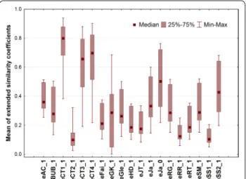
A simple box and whisker plot shows the variability of novel indices: median, interquartile range, minimum and maximum are plotted (Fig. 2).
In Fig. 2, the indices occupy different ranges and cover the domain from zero to (almost) 1. No definite trend can be observed. Hence, the idea seems to be plausible:
all extended similarity indices express the similarity of molecules with error. Then, variance analysis is a suit- able technique to decompose the effects of different fac- tors. The following factors were considered: F2–number (n) of objects (fingerprints) compared, 14 levels: n = 2, 3, …15; F3–role of weighting, two levels: weighted and non-weighted versions; F4–the extended similarity coef- ficients themselves: 19 levels; F5–length of the finger- prints, four levels: m = 10, 100, 1000, 100 000 (F1 being a dummy factor for the cross-validation iterations). Alto- gether 14*2*19*4 = 2128 items (averages of similarity indices) have been decomposed into the above factors.
As expected, the means of the extended indices also show a characteristic zigzag pattern with homogeneous vari- ance (see Additional file 1: Figures S1–S20), which is con- sistent with the results shown in Fig. 1.
The effect of fingerprint length on the overall means is plotted in Fig. 3: here, a definite increasing trend can be seen. Moreover, the variances are also increasing with the fingerprint length (heteroscedasticity). It seems that the curve approximates a limit value (saturation) at a rela- tively small number: ~ 0.38–0.39.
The means of extended similarity coefficients can be decomposed into interaction terms, as e.g. F2*F3. The role of weighting as a function of the multiplicity of fin- gerprint comparisons is illustrated in Fig. 4.
The previously observed zigzag pattern can also be seen here, but the patterns split at n > 3: means of nonweighted coefficients show a damped zigzag pattern. Although
the gap between weighted and non-weighted means increases as the number of compared objects increases, the difference gets smaller between odd and even val- ues of n. The variances remain almost constant, as the multiplicity of comparisons increases. The conclusion
is obvious, there is no use of weighting for binary and ternary comparisons. The largest difference in terms of weighting is for even numbers and 14-ary compari- sons (in the studied range of n at least). Notice how the weighted versions of coefficients have higher means than Fig. 1 Variation of the average (of the absolute value) of all possible n‑ary comparisons over 16 fingerprints of length m = 10 (a, c, e) and
m = 100,000 (b, d, f) for different values of n for the extended Goodman–Kruskal (a, b), extended Sokal‑Michener (c, d) and extended Sokal‑Sneath (e, f) 2 indices
the non-weighted versions. This is an expected result, since while the numerators of both the weighted and non-weighted indices are the same, the denominators of the former are never greater than those of the latter.
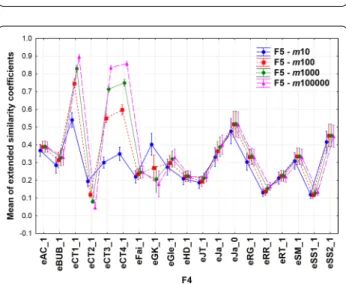
There are many more interactions between the factors, but most of them are hard to perceive. However, the cou- pling between F4*F5 shows a different behavior of the extended similarity coefficients as a function of finger- print lengths (Fig. 5).
The individual coefficients cover different ranges as in Fig. 1 and their variances are also highly divergent.
eCT2_1, eRR_1 and eSS1_1 exhibit small variances, whereas those of eGK_1, eJa_0 and eSS2_1 are higher.
Generally, shorter fingerprints show larger variances. In
fact, most of the means of extended similarity coefficients are insensitive to the fingerprint lengths. However, three of the extended coefficients defined originally by Con- sonni and Todeschini (eCT1_1, eCT3_1 and eCT4_1) exhibit highly diverging behavior as the fingerprint lengths increase, with two more coefficients (eCT2_1 and eGK_1) behaving similarly, but to a lesser extent. The lat- ter two produce a reverse ordering (c.f. color codes) than the highly diverging indices. These behaviors can be eas- ily understood if we look at these indices’ formulas (see Appendix 1: Table 1). In most of the cases, the numera- tors and denominators only include terms that are func- tions of a, b, c, and d. As the fingerprint length increases, these terms also increase in a roughly proportional way, so their ratio will remain approximately constant. In the case of the CT indices, however, we have some “1 + ” terms that break this proportionality, which means that the mean value of these indices will indeed depend on the fingerprint length. This explains why in the limit of infi- nite fingerprint length, eCT1, eCT3, and eCT4 all tend to 1, while eCT2 tends to 0.
The features of the indices have far reaching conse- quences. In the next chapter, we aim to determine which one should be chosen optimally.
Analysis of SRD data
As SRD is a preferable multicriteria optimization tool, it can be advantageously applied to select the best and rec- ommendable indices for further usage. In our example, the total number of fingerprints was 16. The SRD input matrix has been changed as the numbers of compared objects changed from n = 2 to n = 15. The number of rows in the input SRD matrix was given by the binomial coefficients: 16!/[n!*(16-n)!] where 1 < n < 16. The small- est number of rows we considered was 15 for n = 2 and n = 15, then 120 for n = 3 and n = 14, and so on, whereas the largest number of rows was 12 870 for n = 8. The extended similarity coefficients were enumerated in the columns of the SRD input matrix. No data preprocessing was necessary as all coefficients are scaled between 0 and 1.An example SRD result is shown in Fig. 6
The information is represented in such SRD plots as distances from 0 and the random distribution, and the proximity and grouping of the lines. Several extended indices behave similarly (degeneration), coincidence can be seen on some of the lines in case of weighting.
The following factors were considered: F1–variants of sevenfold cross-validation, 2 levels: contiguous and repeated resampling (without and with return, respec- tively); F2–number (n) of compared objects (finger- prints), 14 levels: n = 2, 3, … 15; F3–role of weighting, two levels: weighted and non-weighted versions; F4–the Fig. 2 Box and whisker plot of extended similarity coefficents.
Maximum number of fingerprints to be compared is 16
Fig. 3 Mean of extended similarity coefficients as a function of fingerprint length. The length of the fingerprint is given as numbers of the x axis after m
similarity coefficients themselves: 19 levels; F5–length of the fingerprints: four levels m = 10, 100, 1000, 100 000.
Altogether 2*7*14*2*19*4 = 29 792 SRD values were sub- jected to variance analysis.
Although the ANOVA completed on SRD scores is basically the same as in the case of the mean similarity values, one crucial difference should be mentioned. As SRD is a city block (Manhattan) distance to a gold stand- ard, the smallest SRD value means a better scenario, such a way the best/recommendable indices, number of objects compared, etc. can be revealed and selected.
This feature is not applicable on the mean similarity val- ues (previous section). Hence, the box and whisker plot (Fig. 7) shows some rearrangements as compared to that of the similarity values (Fig. 2).
Fig. 4 The effect of weighting on the means of extended similarity coefficients as a function of compared objects (fingerprints), w = weighted, nw = non‑weighted
Fig. 5 Means of extended similarity coefficients. Line plots
correspond to the length of the fingerprints (F5). The abbreviations of coefficients can be found in Appendix 1
Fig. 6 SRD ordering of extended similarity coefficients for a realistic fingerprint length, m = 1000, weighting was applied, number of objects compared was n = 13. X and left Y axes plot the scaled SRD values between 0 and 100. The Gaussian approximation of the discrete random distribution (~ 60 < SRD < ~ 70) was omitted for clarity. The abbreviations can be found in Appendix 1
Fig. 7 Box and whisker plot for scaled SRD values (between 0 and 100)
Fig. 8 Sum of ranking differences (SRD) scores scaled between 0 and 100 as a function of the number of compared objects (n)
Two indices immediately arise as preferable ones (clos- est to the reference): eBUB_1 and eFai_1, whereas eJa_0 (which includes the 0-similarity counters) has the largest variability. The nice behavior of the eBUB_1 index is in perfect agreement with the properties of the binary BUB index, as observed in our metabolomics study [17].
The dependence on the multiplicity on comparisons preserves the zigzag pattern, but is somewhat distorted (Fig. 8). The essential difference is that the generally decreasing trend has two jumps at n = 3 and n = 14, dis- couraging the usage of these numbers of objects com- pared. The minimum is reached at n = 13, which is therefore suggested as the best number of objects to compare (closest to the reference).
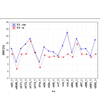
The above statement may be nuanced by the fact that weighting has a different effect on the multiplicity in case of the SRD values (Fig. 9), if n > 3.
While weighting has no influence at the beginning for n = 2 and 3; non-weighted coefficients show a somewhat increasing-alternating trend deviating from the gold standard. Comparison of 14 objects exhibits the highest gap between the weighted and non-weighted scenarios.
In general, weighting is recommended above an n value of three.
Figure 10 shows the effects of weighting on the extended similarity coefficients. Generally, weighting is advantageous (smaller SRD values), and the confidence intervals are so small that they are barely visible (except for eJa_0 non-weighted). It means that all coefficients provided significantly different results, significantly dif- ferent distances from the reference (consensus). There are some cases when weighting plays a subordinate role:
eCT4_1 and eSS1_1. Two indices manifest highly advan- tageous features (close to the reference): eBUB_1 and eFai_1, with and without weighting, alike. Some indices are relatively good, especially in weighted forms, and they are indistinguishable from each other: eGle_1, eJT_1, eJa_1, eRG_1, and eSS_1. The Jaccard-Tanimoto coef- ficient in its extended form is also an acceptable choice, though there are some “better” indices (i.e. more consist- ent with the consensus).
Similarly, equivalent indices can be observed from among the non-weighted ones: eAC_1, eCT1_1, eRT_1 and eSM_1. Finally, the interplay of three factors F2*F3*F5 is presented in Fig. 11: number of compared objects, weighting and fingerprint length. It is under- standable that the smallest fingerprint length produces the smallest SRD values. The realistic 1000 bit-length fin- gerprint has an intermediate position, especially n = 14 is an outlier, still it is recommendable for further usage if using weighting.
Summary and conclusion
The present work introduces a series of new similar- ity indices, which can be applied for the comparison of more than two objects (bitvectors) at once. The essence of the novel extended similarity coefficients is their abil- ity to compare multiple objects at the same time. The features of the average similarity coefficents was stud- ied in detail: the effects of multiplicity, role of weight- ing, and the fingerprint length have also been studied by variance analysis. A multicriteria decision tool (sum of ranking differences) allowed to select the most advanta- geous similarity coefficents. We conclude that in gen- eral, comparing a larger number of objects (n = 12–14) with weighted similarity indices is more advantageous.
Two indices are manifested as highly advantageous (close Fig. 9 Sum of ranking differences scaled between 0 and 100 as a
function of the number of compared objects (n) for weighted and non‑weighted extended similarity indices
Fig. 10 Effect of weighting on the extended similarity coefficients (w = weighted, nw = non‑weighted)
to the reference): eBUB_1 and eFai_1, with and without weighting, alike.
Currently, chemical diversity of a set of molecules is calculated as the mean of all the pairwise similari- ties between the molecules of the set (order O(N2)). The framework that we introduced here provides a new alter- native, which allows to simultaneously compare more than two dichotomous vectors. This scales in order O(N), presenting a tremendous speed gain: this is further dis- cussed in the accompanying paper [22]. Applications include subset selection, clustering, diversity picking or we can even apply this methodology to estimate the diversities of entire compound libraries.
Appendix 1 See Table 1.
Appendix 2: Extended Sokal‑Michener index for quaternary (4‑ary) and quintenary (5‑ary) comparisons
In order to exemplify the work with the new concepts introduced in the manuscript, and to illustrate the work with the n-ary similarity indices, here we present a detailed calculation of the eSM index in two different cases.
4-ary eSM:
To fix ideas, let us compare the following four fingerprints:
a) The first step is to calculate the C4(k) counters, keep- ing in mind that 0≤k≤4:
F1=(10110100) F2=(00100101) F3=(10111001) F4=(00110100)
(2.1) C4(4)=1;C4(3)=2;C4(2)=2;C4(1)=1;C4(0)=2 Fig. 11 Effect of the number of compared objects on (weighted and non‑weighted) extended comparisons of fingerprints with various lengths