Bias in estimates of the classic and incidence-based Jaccard similarity indices: insights from assemblage simulation

(1)

dOi: 10.1556/168.2018.19.3.12

Introduction

Understanding how and why species composition of assemblages varies over space and time has been a focus of ecology for an extended period. This knowledge is also critical for effective biodiversity conservation (Su et al. 2004, Steinitz et al. 2005). The differences in species composition between assemblages are often summarized with a similarity index or distance measure which can be used to measure β-diversity directly (e.g., Legendre et al. 2005) or be further analyzed with multivariate techniques (Legendre and Legendre 2012).

Two challenges arise in estimating the similarity between assemblages (i.e., assemblage similarity), selecting a similarity index and accurately estimating the value of the index selected. Given the subjective nature of similarity, ecologists basically are free to define and choose any similarity index to meet their research goals (Legendre and Legendre 2012).

However, some similarity indices have been found more useful than others in practice (Faith et al. 1987, Cao and Epifanio 2010). It is also known that estimates of similarity indices are often biased (Chao et al. 2005, Cardoso et al. 2009). The bias may distort our perception of assemblage patterns (Cao et al.

2002, Chao et al. 2005) and lead to over- or under-estimating of β-diversity (Condit et al. 2005, Cardoso et al. 2009). This challenge has prompted considerable efforts to develop similarity indices that can be estimated more accurately than those established ones (e.g., Smith et al. 1996, Yue et al. 2001, Chao

et al. 2005, 2006, Engen et al. 2011). I focused on this second challenge in the present study.

When some species missed in samples, estimates of between-assemblage similarity can be biased (Yue et al. 2001, Chao et al. 2005, 2006). However, missing species per se may or may not lead to bias. For example, if missing species have equal chances to be shared by two assemblages or unique, a binary index (e.g., Jaccard Index) will be accurate even at a low sampling level. Therefore, it is how assemblages differ from one another that logically affects the bias in similarity estimates (also see Yue et al. 2001, Chao et al. 2005). Two assemblages may differ in any subsets of species (e.g., random, common or rare) of any sizes. The direction and amount of the bias may therefore vary across pairs of assemblages.

In addition, Engen et al. (2011) reported that the correlation of abundance of individual species between two assemblages was important. However, few studies have systematically in- vestigated into how to characterize assemblage differences and how the differences affect bias in similarity estimates.

The answers to these questions can provide insights into when bias is likely to occur and how to correct it.

A rigorous investigation requires assemblage data that encompass a wide range of species richness, species-abundance distributions, and ß-diversity. Few field sampling datasets meet all these requirements, but simulation provides alternative. One can simulate individual assemblages sepa- rately based on probability models (Chao et al. 2000, Pan et

Bias in estimates of the classic and incidence-based Jaccard similarity indices: insights from assemblage simulation

Y. Cao

Illinois Natural History Survey, Prairie Research Institute, University of Illinois at Urbana-Champaign, 1816 S Oak Street, Champaign, IL 61820, USA. Email: yongcao@illinois.edu; phone: 1 217 244 6847; fax: 1 217 333 6294 Keywords: Assemblage simulation, Beta-diversity, Estimating assemblage similarity, Under-sampling.

Abstract: Similarity indices are often used for measuring b-diversity and as the starting point of multivariate analysis. In this study, I used simulation to examine the direction and amount of bias in estimates of two similarity indices, Jaccard Coefficient (J) and incidence-based J (J^). I design a novel simulation to generate three sets of assemblages that vary in species richness, species-occurrence distributions, and b-diversity. I characterized assemblage differences with the ratio of [proportion of rare species in all shared species / proportion of rare species in all unshared species] (i.e., PR_ss/PR_us) and the Pearson’s correlation in the probabilities of shared species between two assemblages (i.e., share-species correlation). I found that J was subject to strong positive or negative bias, depending on PR_ss/PR_us. J^ was mainly subject to negative bias, which varied with share-species correlation. In both indices, bias varied substantially from one pair of assemblages to another and among datasets. The high variation in the bias across different comparisons of assemblages may compromise b-diversity estimation established at low sampling efforts based on the two indices or their variants.

Abbreviations: J = the classic Jaccard Coefficient, J^ = the incidence-based Jaccard Coefficient adjusted for unseen species, NSS = the Number of Shared Species by two assemblages, P_ij= occurrence probability of Species j at a random sample unit in Assemblage i, PRss = the Proportion of Rare species out of all Shared Species by two assemblages, PRus = the Proportion of Rare species out of all Unshared Species by two assemblages, SOD = Species-Occurrence Distribution – a plot of relative occurrence frequency of species against their ranks (from common to rare), TSR = the Total number of species in a pair of assemblages.

(2)

al. 2009) or species-abundance distribution models (Cardoso et al. 2009). However, previous simulations are not always ecologically realistic, for instance, assuming homogeneous, random or normal distributions of species probability, and no correlation in species probability or abundance among assemblages. In the present study, I generated three series of assemblages that mimic commonly-observed ecological changes over space or time. In particular, I systematically manipulated the correlation in the probabilities of occurrence for shared species between two assemblages to create a range of ß-diversity.

Among numerous similarity indices available (Legendre and Legendre 2012), I focused on two binary indices. The Jaccard Index (J) is most commonly used for measuring b- diversity (Baselga 2010, Carvalho et al. 2012) and multivariate analysis of binary data. The incidence-based J adjusted for unseen shared species incidences (J^) (Chao et al. 2005) is relatively new, but also increasingly adopted. Both indices measure the ratio between shared and all species, but J^ is based on the number of species incidence regardless whether the incidences are from one or multiple species whereas a species is only counted once in J. Therefore, they measure similarity differently and should be treated as two similarity indices.

My specific goals here include 1) establishing a technical framework to simulate a series of diverse assemblages and manipulate assemblage differences, 2) evaluating how bias in the two indices is related to species-probability correlation between assemblages and the portioning of missing species between shared and unshared species.

Methods

Charactering assemblage relationships

I defined a few terms to describe how missing species in samples (rare species) are allocated between two assemblages and used them to manipulate their differences later.

P_ij= Probability of occurrence of species j at a random sample unit in Assemblage i;

Unshared rare species = species present in one assemblage only and with P_ij <0.05;

Shared rare species = species present in both assemblages with P_1i× P_2i< 0.05;

PRss = the Proportion of Rare species out of all Shared Species;

PRus = the Proportion of Rare species out of all Unshared Species.

Recognizing that any definition of rare species is arbitrary, I considered those unshared species with 0.05 probability of occurrence to be rare. Whether a shared species is “rare” is dependent on the product of the probabilities of the species in both assemblages (i.e., P1i ×P2i). If the conduct is < 0.05, the species was considered as shared rare species. I also used the ratio PR_ss/PR_usto measure the relative pace of shared and unshared rare species being added to assemblage comparison

when sampling effort increases, something that may be critical for the bias of J estimates. In examining three intensive field datasets of aquatic assemblages, Cao (unpublished data) found PR_ss ranging from 0.25 to 0.65, PR_ss/PR_us from 0.44 to 2.86. I incorporated these observations into simulation later.

J^ only considers shared species in its adjusting for un- seen species (see Appendix 1) and therefore should not be affected by PRss/PRus. Instead, I calculated the Pearson’s correlation of the probability in shared species between two assemblages or simply share-species correlation. In examining three field sampling datasets mentioned earlier, Cao (unpublished data) found shared-species correlation in relative frequency varying from -0.90 to 0.80, and I manipulated assemblage differences later to achieve a similar range.

Generating series of assemblages and manipulating their differences

I generated three series of assemblages based on three types of species-occurrence distribution (SOD) models (Appendix 2) (Cao et al. 2007). Negative-exponential SOD predicts many species and most species to be rare, logistic SOD relatively low numbers of species and most species being common, and linear SOD intermediate numbers of species, and rare and common species to be equal. The model parameters used fell within the ranges observed from field data (Cao et al. 2007). In assembling individual assemblages into an ecological series, I manipulated the overlap of species composition among assemblages and the shared-species correlation in each series of assemblages (Fig. 1).

1) Series A - a set of species-rich assemblages. I simulated a series of assemblages that might mimic a set of tropical forest plots along a strong environmental gradient. I used a negative-exponential type of SOD to generate the probabilities of 300 species for one assemblage (A1) (Table 1). By replacing 10%, 20%,..., 100% of randomly selected species from A1 with new species that have the same probabilities, I created 10 more assemblages (A2-A11) with 600 species in total (see Appendix 3). I then manipulated the correlation of shared species by randomizing the probabilities of shared species by 0% - 100% at the intervals of 10% in A2-A11, respectively. As a result, all 11 assemblages have identical species richness (300) and SOD.

2) Series B - a set of successional assemblages. I created a second series of assemblages to mimic a succession series (Table 1). An assemblage often starts with a few generalist species in a new habitat and, over time, new species move in while some pioneer species disappear and species dominance tends to reduce. I created the first assemblage (B1) of 15 species with a logistic SOD model. The 2^nd assemblage (B2) was created by dropping 1/3 species randomly selected in B1 and adding 15 new ones. The probabilities of 25 species in B2 were generated with a new logistic SOD model, and the 10 species retained from B1 were given higher probabilities, a step that leads to a high share-species correlation. Two more assemblages (A3-A4) were created by dropping 1/3 species of the previous one, but based on linear and negative-expo-

(3)

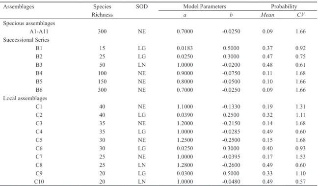
Table 1. Model parameters used for generating three sets of simulated assemblages. NE = negative-exponential type of species-occur- rence distribution or SOD, LG = logistic type of SOD, LN = linear type of SOD, a = the probability of the most common species, b = a parameter controlling the rate at which the probability of subsequent species decreases, see Appendix 2 for more details.

Figure 1. Framework of simulating a set of assemblages used to evaluate the accuracy of similarity indices.

Assemblages Species SOD Model Parameters Probability

Richness a b Mean CV

Specious assemblages

A1-A11 300 NE 0.7000 -0.0250 0.09 1.66

Successional Series

B1 15 LG 0.0183 0.5000 0.37 0.92

B2 25 LG 0.0250 0.3000 0.47 0.75

B3 50 LN 1.0000 -0.0200 0.48 0.61

B4 100 NE 0.9000 -0.0750 0.11 1.68

B5 150 NE 0.8000 -0.0500 0.10 1.66

B6 300 NE 0.7000 -0.0250 0.09 1.66

Local assemblages

C1 40 NE 1.1000 -0.1330 0.19 1.31

C2 40 LG 0.0390 0.2500 0.32 1.11

C3 35 NE 1.2000 -0.2150 0.14 1.68

C4 35 LG 1.0000 -0.0285 0.49 0.60

C5 30 NE 1.2500 -0.2500 0.15 1.68

C6 30 LG 0.0250 0.3000 0.40 0.93

C7 25 NE 1.0000 -0.0395 0.17 1.53

C8 25 LN 1.2800 -0.2600 0.49 0.60

C9 20 LG 0.0300 0.5000 0.33 1.10

C10 20 LN 1.0000 -0.0480 0.49 0.57

22 Fig. 1. Framework of simulating a set of assemblages used to evaluate the accuracy of similarity indices

Choosing the number of assemblages and richness range for a series

Assigning richness and SOD-type to each assemblage

Setting the species overlap among assemblages

Manipulating the correlation in shared species between assemblages

Creating 10,000 spatial units for each assemblage based on uniform random distribution

Drawing 10 subsets of n units (10 n  640)

Calculating the average values ofJ,J^ and NSS from 1010 combinations

Calculating the true value ofJ and J^ for each pair of assemblages

Calculating the relative bias of estimates in J and J^

Calculating the values of PRss, PRus, and shared- species correlation

Relating the relative bias in J and J^ estimates to PRss, PRus, NSS, and/or shared-species correlation (r)

(4)

nential SODs, respectively, and with 50 and 100 species in total (Appendix 3). Again, the retained species were given high probabilities. Assemblage B5 (150 species) and B6 (300 species) were generated in the same way, but based on negative-exponential SODs and the probabilities of the species shared by these two assemblages were assigned randomly, a step that reduces shared-species correlation.

3) Series C - a set of local assemblages. A local assem- blage typically contains a subset of the regional species pool (Angermeier and Winston 1998). I first created a 100-species pool with a negative-exponential type of SOD, and then drew 10 random subsets of 20-40 species with replacement to ob- tain a range of overlaps in species composition among assemblages (Table 1, Appendix 3). The probabilities of species in each of the 10 assemblages (C1-C10) were regenerated with different SOD models (Table 1). To manipulate shared- species correlation, I first ranked the occurrence frequencies of all 100 species across the 10 assemblages, and then assigned a P_i value to a species in line with its regionally com- monness so that regionally common species were also locally common. I then reduced the correlation to varying extents by randomizing the probabilities of shared species by 100% in C1 - C2, 75% in C3-C4, 50% in C5-C6, 25% in C7-C8, and 0% in C9-C10, respectively.

Sampling scheme

I generated 10,000 replicate samples for each assemblage based on the specific SOD of an assemblage with the uniform random distribution (Cao et al. 2007). Given N species present in an assemblage, I first generated 10,000 rows of random numbers and each row has N elements (e_ij, 1 ≤ i ≤ N, 1 ≤ j ≤ 10,000). If the probability of Species i (Pi) generated based a given SOD model (N species) is equal to or greater than eij in a row we replaced eij with 1, otherwise with 0. This step turned each row into a random replicate of species presence-absence. Ten subsets of replicates were drawn without replacement from this replicate pool with 10, 20, 40, 80, 160, 320, or 640 replicates per subset (0.1 – 6.4% of the pool). To estimate J, a subset of replicates was pooled into a single composite sample, but all replicates in a subset were kept separate and used to estimate J^. The values of J and J^

estimated for 10 × 10 combinations of the subsets from two assemblages were averaged (Fig. 1). There are 55, 45, and 15

possible pairs of assemblages in Series A-C, respectively. A1 and A11 shared no species and this pair was excluded from further analysis.

Data analysis

Bias is typically calculated as (estimates – the true value).

The theoretical ranges of J and J^ are all 0-1, however, the actual ranges differ from one dataset to another and between J and J^ (Table 2). The ecological significance of a given bias appears to vary with similarity index and dataset. For example, a bias of -0.1 may be acceptable when the true value is 0.9, but not if the true value is 0.2. I therefore also normalized the bias as ([estimate – true value] / true value) as in Chao et al. (2005, 2006), and referred to it as relative bias. I com- bined the 10000 replicates into a whole assemblage and used it to calculate the true value of J and J^ for each pair of assemblages. When the true value is very low, sampling errors often led to extremely high relative bias. I therefore excluded those comparisons with the true value of < 0.1. As a result, one comparison was dropped from each of Series A and C, and eight comparisons from Series B. In addition, Chao et al. (2005) suggested at least 10 shared species sampled for appropriate use of J^. I therefore also counted the number of shared species (NSS) in each comparison.

The difference in the bias between J and J^ was tested with Wilcoxon Test (Systat12, Systat Software, Inc. 2007). The relationships of relative bias in J estimates with PR_ss/PR_us, and in J^ with PRss and the shared-species correlation were exam- ined by plotting the bias against each of the factors.

Results

Characteristics of three series of assemblages

In Series-A, assemblage similarity varied widely (0.10 ≤ J ≤ 0.82, 0.08 ≤ J^ ≤ 0.89) and so did shared-species correla- tion (-0.11 ≤ Pearson r ≤ 0.99) and the total number of species in a pair of assemblages (330-540), but PR_rs/PR_us ranged moderately (1.05 - 1.65, Table 2). In comparison, Series-B assemblages differed more substantially in total species richness in a pair (30-350), shared-species correlation (-0.35 ≤ r

≤ 0.98), and PR_ss/PR_us (0.56-1.89) while the true similarity values fell into low-medium range (0.12 - 0.39 in J, 0.08 - Table 2. Ranges of five characteristics that may affect the estimation of the Jaccard Coefficient (J) and Chao’s Incidence-based J (J^) and the true values of these two indices in three datasets (those comparisons with the true value < 0.1 excluded). Rare species are defined as those with occurrence probability of ≤ 0.05 for non-shared species and the conduct of probabilities ≤ 0.05 for shared species.

The proportions of rare species in all shared species and in all unshared species are referred to as PR_ssand PR_us, respectively, and the total number of species in a pair of assemblages compared as TSR, and the correlation of shared species between two assemblages is measured with Pearson correlation r.

Dataset Number of

comparisons TSR Shared-species

correlation (r) PRss PRus PRss/PRus True value

of J True value of J^

Series A 52 330 - 540 -0.11-1.00 0.83- 0.99 0.53 - 0.80 1.05 - 1.65 0.10 - 0.82 0.08- 0.89 Series B 8 30 - 350 -0.35 - 0.98 0.14 - 0.99 0.10 - 0.77 0.56 - 1.89 0.12 - 0.39 0.08 - 0.56 Series C 44 34 - 58 -0.19 - 0.99 0.00 -0.80 0.07- 0.85 0.30 - 1.95 0.10- 0.53 0.19 - 0.81

(5)

0.56 in J^, Table 2). Series-C assemblages were associated with moderate variation in total species richness in a pair, high variation in PRrs/PRru (0.30-1.95), and shared-species correlation (-0.19 ≤ r ≤ 0.99), and low-intermediate or high assemblage similarity (0.10- 0.53 in J, 0.19 - 0.81 in J^, Table 2). The three series thus captured a wide range of assemblage variation as originally planned.

Bias in estimates of J and J^

The bias in estimates of J and J^ varied greatly among pairs of assemblages and datasets (Table 2). The average ab- solute bias (i.e., |bias|) in J was higher than in J^ in all series (p < 0.05 for A and C, Wilcoxon Tests), although J was less biased in some pairs of assemblages.

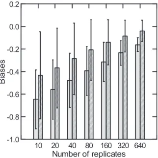
The relative bias (and bias) always decreased with increasing sampling effort, but J estimates on average remained to be more biased (see Fig. 2 for example). The relative bias also varied substantially across pairs of assemblages, ranging from -0.82 to 0.80 in J, and from -0.68 to 0.10 in J^ at 10 replicates, a sampling effort most likely used in practice, and differed among the three series of assemblages, all negative in Series-A, both negative and positive in Series-B and C (Fig.

3). In addition, the bias in J^ was often negative, and when positive, it was small. In comparison, relative bias in J estimates could be strongly positive or negative (Fig. 3). Overall, the direction and amount of bias in both J and J^ estimates are dependent on the assemblages compared.

23 Fig. 2. Average relative bias in estimates of the Jaccard Index (J) (left in each group of bars) and the Chao’s adjusted index (J^) (right) (with 95% confidence limits at 10-640 replicates in Series A with Y-axis ranging from negative to zero and positive.

10 20 40 80 160 320 640

Number of replicates

-1.0

-0.8 -0.6 -0.4 -0.2 0.0 0.2

Bi as es

Figure 2. Average relative bias in estimates of the Jaccard Index (J) (left in each group of bars) and the Chao’s adjusted index (J^) (right) (with 95% confidence limits at 10-640 replicates in Series A with Y-axis ranging from negative to zero and positive).

Figure 3. Distributions of relative bias in estimates of J (circle) and J^ (cross) among all pairs of assemblages that have the true value of J greater than 0.1 in Series A, B, and C of simulated assemblages.

24 Fig. 3. Distributions of relative bias in estimates of J (circle) and J^ (cross) among all pairs of assemblages that have the true value of J greater than 0.1 in Series A, B, and C of simulated assemblages.

-1.0 -0.8 -0.6 -0.4 -0.2 0.0 0.2 0.4 0.6 0.8 1.0

A

B

C

Distributions of relative bias

-1.0 -0.8 -0.6 -0.4 -0.2 0.0 0.2 0.4 0.6 0.8 1.0

A

B

C

Distributions of relative bias

-1.0 -0.8 -0.6 -0.4 -0.2 0.0 0.2 0.4 0.6 0.8 1.0

A

B

C

Distributions of relative bias

(6)

Effects of PR_ss/PR_us and shared-species correlation on relative bias

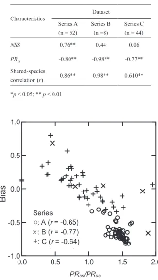
Relative bias in J estimates quickly decreased with increasing PR_ss/PR_us (-0.64 ≤ r ≤ -0.77) and particularly in Series A and C (p < 0.01) (Fig. 4). Because the bias was always negative in Series A, the negative correlation means that the underestimation of J became more severe with increasing PRss/PRus ratio. The bias could be negative or positive in Series B and C, and the strong negative correlation in these cases therefore means positive bias decreasing when the ratio increased from 0 to 1, and negative bias increasing when the ratio further increased above 1.

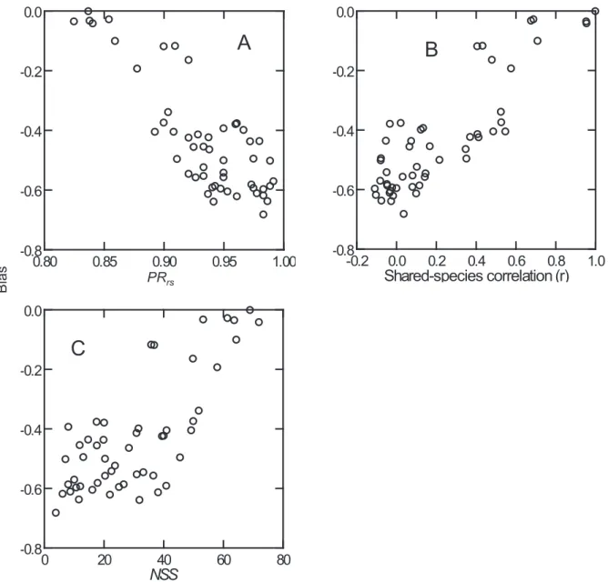
The negative relative bias in J^ estimates increased with Pss (-0.77≤ r ≤ -0.98, p<0.01) and decreased with shared-species correlation (0.61 ≤ r ≤ 0.97, p < 0.01) (Table 3 and Fig.

5). The bias was also reduced with increasing the number of shared species sampled (NSS) in Series A (r = 0.76, p < 0.01), but not in Series B and C (r = 0.06-0.43, p > 0.05). It was also noted that relative bias in J^ estimates was often sub- stantial even when 10 shared species were sampled. A much greater number of shared species (e.g., >70) was needed to effectively reduce the bias (Fig. 5C). In summary, bias in J and J^ estimates was related to different aspects of assem- blage variation.

Discussion

Assemblage similarity underlies many concepts, such as b-diversity (e.g., Baselga 2010, Carvalho et al. 2012) and provides the starting point for multivariate analyses (Legendre and Legendre 2012). However, biased estimates are a major concern (e.g., Chao et al. 2005, 2006, Carsodo 2009). In the present study, I used a range of simulated assemblages to evaluate the accuracy of J and J^ estimates. My analysis not only revealed some important sampling properties of these two indices, but also identified the factors that strongly affect the accuracy. The simulation framework developed here is also useful to evaluate other measures of similarity and b- diversity.

I first showed that bias in estimates of both indices could vary greatly from one pair of assemblages to another.

Negative bias in estimates of J was generally assumed (Chao et al. 2005, 2006), and did occur more commonly and more severely in my simulation than positive bias. However, the latter could be strong and common under certain circum- stances (e.g., Series C in the present study). This finding should not be surprising because the bias depends on PRss/ PR_us ratio (Fig. 4) and there is no ecological basis for assuming that this ratio has always to be ≥ 1, i.e., shared rare species added to samples equally as or more quickly than unshared species when sampling continues. Positive bias in J estimation was rarely reported for field datasets, probably because intensive assemblage surveys are rare, but Holtrop et al.

(2010) observed several cases of positive bias in comparing stream fish assemblages. A meta-analysis based on intensive surveys is needed to assess the occurrences of positive bias for this and other similarity indices. It is also worth testing

whether the value of PR_ss/PR_us calculated based on samples could indicate the direction and amount of bias in J estimates.

Bias in J^ estimates in my simulation was generally negative (Table 2), and smaller on average than in J (Fig. 3), an observation supported by Chao et al. (2005, 2006) and Cao and Epifanio (2010). However, this higher accuracy may not hold for specific comparisons, as shown in the present study.

Chao et al. (2005) found J^ highly resistant to under-sampling in their simulation, but estimates of J^ were severely biased in my simulation when shared species were weakly or negatively correlated (Fig. 5A-B). This result is not surprising. A weak or strongly negative shared-species correlation means that many or most shared rare species in one assemblage are common in another. Missing those shared rare species in sam- Table 3. Correlations of the relative bias in estimates of Chao’s Incidence-based Jaccard Coefficient (J^) at 10 replicates with three factors: proportion of rare species in all shared species (PRrs), the correlation of probabilities in shared species measured with Pearson’s r, and the number of shared species recorded (NSS) at 10 replicates in three datasets.

Figure 4. Relationships of relative bias in J estimates with the ratio between the proportions of rare species in all shared species (PRss) and in all unshared species (PRus) in three simulated datasets.

Dataset Characteristics

Series A (n = 52)

Series B (n =8)

Series C (n = 44)

NSS 0.76** 0.44 0.06

PR_ss -0.80** -0.98** -0.77**

Shared-species

correlation (r) 0.86** 0.98** 0.610**

*p < 0.05; ** p < 0.01

Fig. 4. Relationships of relative bias in J estimates with the ratio between the proportions of rare species in all shared species (PRss) and in all unshared species (PRus) in three simulated datasets.

3 (r=-0.64) 2 (r=-0.77) 1 (r=-0.65) Dataset

0.0 0.5 1.0 1.5 2.0

-1.0 -0.5 0.0 0.5 1.0

Bias

PRss/PRus

Series

○

: A (r = -0.65)



: B (r = -0.77)

+

: C (r = -0.64)

(7)

ples will lead to a failure of recognizing them as the shared species and thus contribute to negative bias far more than missing shared species being rare in both assemblages in calculating J^. However, the number of shared singletons (i.e., f₊₁ or f₁₊in Appendix 1) in samples would be low in this case because the species are common in one of the two assemblages compared. This low number leads to inadequate adjustment in J^ and then much of negative bias will remain.

In contrast, strong and positive shared-species correlation means that shared species missed are often rare in both assemblages. These missing species are weighted lightly in J^

and their effects also can be better adjusted because the high values of f+1 and f1+ in this case. As a result, one can expect less bias. What is not clear is whether an estimate of the correlation based on samples can indicate the amount or direction of bias, a question that needs to be addressed in future studies.

A more important observation in the present study is that bias at a given sampling effort was highly variable, from practically none in some cases to strongly positive or negative in other cases (Figs. 3-5). When a similarity index is used to measure b-diversity, negative or positive bias will lead to over- or under-estimation of b-diversity. b-diversity patterns estimated at a low sampling effort therefore require caution to interpret. As J and J^ are mathematically related to the classic and incidence-based Sørensen Index, respectively, and the results should be directly applicable to the last two indices.

It also appears reasonable to expect that other classic binary similarity indices would be sensitive to PR_ss/PR_us; similarly, abundance-based similarity indices (e.g., Bray-Curtis Index) are likely to be sensitive to the correlation of abundance in shared species between assemblages, a topic that warrants investigation in the future.

Fig. 5. Relationships of relative biases in J^ estimates with the proportion of rare species in all shared species (PR

ss

) (Panel A), and shared-species correlation (Panel B), and the number of shared species sampled (NSS) (Panel C) in comparing 11 assemblages of Series A.

0 20 40 60 80

NSS -0.8

-0.6 -0.4 -0.2 0.0

0.80 0.85 0.90 0.95 1.00

-0.8 -0.6 -0.4 -0.2 0.0

-0.2 0.0 0.2 0.4 0.6 0.8 1.0 Shared-species correlation (r) -0.8

-0.6 -0.4 -0.2 0.0

PR_rs

Bias

A B

C

Figure 5. Relationships of relative biases in J^ estimates with the proportion of rare species - shared species (PRss) (Panel A), and shared-species correlation (Panel B), and the number shared species sampled (NSS) (Panel C) in comparing 11 assemblages of Series A.

(8)

Finally, I like to highlight some strength and constrain of the simulation framework used in the present study (Fig.

1). Comparing with previous simulations, this framework is more ecologically realistic in terms of species-occurrence distribution. It also provides a great flexibility to manipulate the share-species correlations and species overturn rate. By replacing SOD models with species-abundance distribution models (e.g., log-normal and log-series), one can generate species-abundance data to examine the accuracy of abundance-based similarity indices, such as Bray-Curtis Index.

However, it is not clear how frequently the relationships simulated occur in nature. Future studies should examine the variation of PR_ss/PR_usand shared-species correlation based on intensive field data in relation to habitat diversity, taxo- nomic groups, and spatial scales in assemblage analysis.

Conclusion

The direction and amount of the bias in J is closely related to how rare species are partitioned between groups of shared and unshared species. The bias of J^ estimates strongly depends on the correlation of probabilities in shared species. J estimates are more often subject to bias than J^ estimates. The adjustment for unseen species in J^ appeared less effective when the probabilities of shared species by two assemblages are weakly or negatively correlated. The bias of estimates in the two indices can be highly variable across pairs of assemblages and datasets and thus the b-diversity patterns established at a low sampling effort require caution to interpret.

Acknowledgements. The author gratefully acknowledges the constructive comments of P. Minchin on an earlier draft.

This study was supported by Illinois Natural History Survey, University of Illinois. Discussions with C.P. Hawkins and J.

Van Sickle helped the author to frame this study.

References

Baselga, A. 2010. Partitioning the turnover and nestedness compo- nents of beta diversity. Glob. Ecol. Biogeogr. 19:134-143.

Cao, Y. and J. Epifanio. 2010. Quantifying the responses of macroin- vertebrate assemblages to simulated stress: are more accurate similarity indices less useful? Methods Ecol. Evol. 1:380-388.

Cao, Y., C.P. Hawkins, D.P. Larsen and J. Van Sickle. 2007. Effects of sample standardization on mean species detectabilities and estimates of relative differences in species richness among assemblages. Am. Nat. 170:381-385.

Cao, Y., D.P. Larsen, R.M. Hughes, P. Angermeier and T. Patton.

2002. Sampling efforts affect multivariate comparisons of stream assemblages. J. N. Am. Benthol. Soc. 21:707-714.

Cardoso, P., P.A.V. Borges and J.V. Veech. 2009. Testing the perfor- mance of beta diversity measures based on incidence data: the robustness to undersampling. Divers. Distrib. 15:1081-1090.

Carvalho, J.C., P. Cardoso and P. Gomes. 2012. Determining the relative roles of species replacement and species richness differences in generating beta-diversity. Glob. Ecol. Biogeogr. 21:760-771.

Chao, A., R.L. Chazdon, R.K. Colwell and T.J. Shen. 2005. A new statistical approach for assessing similarity of species composition with incidence and abundance data. Ecol. Lett. 8:148-159.

Chao, A., R.L. Chazdon, R.K. Colwell and T.J. Shen. 2006.

Abundance-based similarity indices and their estimation when there are unseen species in samples. Biometrics 62:361-371.

Chao, A., W. Hwang, Y.C. Chen and C.Y. Kuo. 2000. Estimating the number of shared species in two communities. Statistica Sinica 10:227-246.

Condit, R., R. Perez, S. Lao, S. Aguilar and A. Somoza. 2005.

Geographic ranges and β-diversity: discovering how many tree species there are where. Biologiske Skrifter Kongelige Danske Videnskabernes Selskab. 55:57-71.

Engen, S., V. Grøtan and B-E. Sæther. 2011. Estimating similarity of communities: a parametric approach to spatial-temporal analysis of species diversity. Ecography 34:220-231.

Faith, D.O., P.R. Minchin and L. Belbin. 1987. Compositional dis- similarity as a robust measure of ecological distance. Vegetatio 69:53-68.

Holtrop, A.M., Y. Cao and C.R. Dolan. 2010. Estimating sampling effort required for characterizing species richness and site-to- site similarity in fish assemblage surveys of wadeable Illinois streams. T. A. Fish. Soc. 139:1421-1435.

Legendre, P., D. Borcard and P.R. Peres-Neto. 2005. Analyzing beta diversity: partitioning the spatial variation of community composition data. Ecol. Monogr. 75:435-450.

Legendre, P. and L. Legendre. 2012. Numerical Ecology. 3^rd Edition, Elsevier, New York.

Pan, H.Y., A. Chao and W. Foissner. 2009. A non-parametric lower bound for the number of species shared by multiple communities. J. Arg. Biol. Envir. St. 14:452-468.

Smith, W., A.R. Solow, and P.E. Preston. 1996. An estimator of species overlap using a modified beta-binomial model. Biometrics 52:1472-1477.

Steinitz, O., J. Heller and A. Tsoar. 2005. Predicting regional patterns of similarity in species composition for conservation planning.

Conserv. Biol. 19:1978-1988.

Su, J.C., D.M. Debinski, M.E. Jakubauskas and K. Kindscher. 2004.

Beyond species richness: Community similarity as a measure of cross-taxon congruence for coarse-filter conservation. Conserv.

Biol. 18:167-173.

Yue, J., M.K. Clayton and F.C. Lin. 2001. A nonparametric estimator of species overlap. Biometrics 57:743-749.

Received June 13, 2018 Revised November 26, 2018 Accepted December 3, 2018

Appendices

Appendix 1. Two similarity indices tested.

Appendix 2. Species occurrence distribution models.

Appendix 3. Conceptual relationships among the simulated assemblages in Series-A, B, and C created based on different species-occurrence distributions.

The file may be downloaded from www.akademiai.com.