Accelerating Convergence of Fluid Dynamics Simulations with Convolutional Neural Networks

(1)

Cite this article as: Hajgató, G., Gyires-Tóth, B., Paál, Gy. "Accelerating Convergence of Fluid Dynamics Simulations with Convolutional Neural Networks", Periodica Polytechnica Mechanical Engineering, 63(3), pp. 230–239, 2019. https://doi.org/10.3311/PPme.14134

Accelerating Convergence of Fluid Dynamics Simulations with Convolutional Neural Networks

Gergely Hajgató^1*, Bálint Gyires-Tóth², György Paál¹

1 Department of Hydrodynamic Systems, Faculty of Mechanical Engineering,

Budapest University of Technology and Economics, H-1521 Budapest, P.O.B. 91, Hungary

2 Department of Telecommunications and Media Informatics, Faculty of Electrical Engineering and Informatics, Budapest University of Technology and Economics, H-1521 Budapest, P.O.B. 91, Hungary

* Corresponding author, e-mail: ghajgato@hds.bme.hu

Received: 02 April 2019, Accepted: 16 May 2019, Published online: 27 May 2019

Abstract

A novel technique to accelerate optimization-driven aerodynamic shape design is presented in the paper. The methodology of optimization-driven design is based on the automated evaluation of many similar shapes which are generated according to the output of an optimization algorithm. The vast amount of numerical simulations makes this process slow but the resource-intensive simulation part can be changed to so-called surrogate models or metamodels. However, there isn’t any guarantee of this solution’s accuracy.

The motivation of this work was to develop an acceleration method to speedup optimization sessions without losing accuracy.

Accordingly, the numerical simulation is kept in the pipeline but it is initialized with a velocity field that is close to the expected solution.

This velocity field is generated by a predictive initializer that is based on a convolutional deep neural network. The network has to be trained before using it for initializing numerical simulations; the data generation, the training and the testing of the network are described in the paper as well.

The performance of predictive initializing is presented through a test problem based on a deformable u-bend geometry. It has been found that the speedup in the convergence speed of the numerical simulation depends on the resolution of the predictive initializer and on the handling of velocities in the near-wall cells. A speedup of 13 % was achieved on a test set of 500 geometries that were not seen by the initializer before.

Keywords

predictive initialization, CFD initialization, deep learning, convolutional neural networks, metamodeling

1 Introduction

Modern design methods in mechanical engineering heav- ily rely on shape optimization as the accessible computational resources are getting bigger. This is especially true in the field of aerodynamic shape design, where diverse products are constructed with the aim of automated optimization techniques. These methods have proven their usefulness in many fields, however, the design process itself is still slow. Several techniques are available to surrogate the time-consuming part of the optimization but at the expense of accuracy. This paper presents a method wherewith the design process can be accelerated without making a compromise on precision. Besides, the presented metamodel works with a parameter-free representation of the shape which could be beneficial in specific cases.

The basic building blocks of an optimization-driven design framework are the parameterized computer model of the geometry, an evaluation method and an optimization algorithm. In such a setting, the optimization algorithm tries to find the global extrema of the return value of the evaluation by varying the descriptive parameters of the geometry.

In aerodynamic shape design, the objective is based mostly on some macroscopic aerodynamic parameter of the shape, e.g. hydraulic efficiency or drag force coefficient or a combination of such values, etc. Therefore, a computational fluid dynamics (CFD) solver has to be utilized to model the underlying physics and to calculate the objective according to a specific shape. Evolutionary algorithms are used most frequently to find the empirical global extrema

(2)

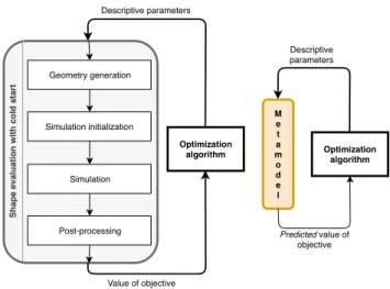
of the objective function according to [1]. The schematic of such a framework is depicted on the left side of Fig. 1.

Besides, gradient-based algorithms can be used when the objective function is expected to be smooth. In such cases, state-of-the-art optimization algorithms involve adjoint CFD-techniques to compute the sensitivity of the flow field to the geometry [2].

Considering time, no matter what the optimization technique is, the bottleneck of the process is the evaluation of the shape, namely the runtime of the CFD solver.

This drawback led to the rise of metamodeling in aerodynamic shape optimization. Metamodels completely surrogate the “accurate” simulation with a function approximator in the optimization process, by mapping the parameterization of the geometry to the objective value directly. Such a framework is depicted on the right side of Fig. 1.

The time-consuming numerical simulation is omitted this way but the accuracy is sacrificed for speed, that may lead to qualifying an improper shape as the optimum.

Another drawback of using a metamodel comes up when the parameterization of the geometry has to be changed.

This happens when the optimum shape lies on the boundary of the parameter set¹ or the shape constraints are changed for some reason. In these cases, the already fitted metamodel is useless with the new parameterization, thus, new CFD cal- culations have to be executed to re-fit the metamodel.

A novel method based on deep learning is presented here, wherewith the CFD simulations of an optimization session can be accelerated without losing accuracy, and the accelerator can be re-used even if the parameterization of the geometry is changed. The schematic of an optimization-driven design framework using the proposed model is depicted in Fig. 2.

2 Related work

State-of-the-art shape optimization algorithms exhaust the benefits of metamodeling but the metamodel has to be fitted prior to the optimization session. Generating samples to fit metamodels is often conducted with design and analysis of computer experiments (DACE) techniques. DACE is originated from the design of experiments (DOE) and was introduced in [3]. While DOE methods assume that random error is present in the observations, DACE methods take into account that the results of computer simulations have mostly deterministic error and are repeatable.

1 This suggests that an even better shape lies outside the original boundaries.

Kriging [4] and the response surface model are proposed in [3] as metamodels for computer simulations. Indeed, these methods were used successfully in [5] to optimize the shape of a helicopter rotor-blade, described by 31 parameters.

Feedforward artificial neural networks (ANN) are named as good candidates for approximating nonlinear response surfaces in [6]. Besides, a comprehensive over- view of optimization and metamodeling techniques is given as well. Kriging and response surface models are also mentioned here, and their performance is held similar in design optimization. Simpson et al. [6] also emphasize

Fig. 1 Schematic diagram of optimization-driven aerodynamic shape design (left side) and the same but using metamodel (right side). Cold start means, that the simulation is initialized conventionally with a

zero velocity field.

Optimization algorithm

Predicted value of objective Descriptive parameters

Me at mo de l

Shape evaluation with cold start

Optimization algorithm Geometry generation

Simulation initialization

Simulation

Post-processing

Value of objective Descriptive parameters

Fig. 2 Schematic diagram of optimization-driven aerodynamic design with warm start of the simulation.

Shape evaluation with warm start

Optimization algorithm

Value of objective Descriptive parameters

Geometry generation

Simulation initialization

Simulation

Post-processing Solution prediction

(3)

that the descriptive parameters of the model should be screened when their number is large.

The drawback of screening is mentioned in [7], wherein the uncertainty of metamodels is presented among several real-life optimization problems as well. Screening is a class of techniques, wherewith the unimportant parameters of an optimization problem can be identified in order to reduce the parameter set during optimization. As mentioned in [7], screening can hide the optimum if the response function of the problem is sensitive to a specific parameter only near the optimum. Thus, the best practice is to finish the optimization involving all the original parameters and to omit the metamodel that was fitted to the reduced parameter set.

Simpson et al. [8] give an extensive review on DACE methods in design optimization with the most import- ant milestones in the development of such techniques.

Besides, the state-of-the-art solutions are presented there and the combination of various metamodels is stated as a robust estimator to surrogate the simulation based on the physical model.

The book of Thévenin and Janiga [1] summarizes the individual work of many authors in the field of design optimization with computational fluid dynamics. Different optimization algorithms, some metamodeling techniques and some DOE methods are described as well. The two- level optimization framework presented by René A. Van den Braembussche involves artificial neural networks to predict the fitness of a new individual in a genetic algorithm, and only a fraction of the individuals is evaluated with the computationally intensive numerical solver.

The basics of feedforward ANNs are also described here and Braembussche presents a study on the effect of fitting an ANN on randomly sampled data over fitting the same network on data generated with a full factorial design. The latter performs better in terms of “global error” but the meaning of this metric is not described.

Response surface models, kriging and feedforward ANNs have proven to be useful in the field of metamodeling-assisted design optimization (among others) and some of them are available even in commercial software nowadays. Though new techniques have been invented and many improvements have been done, state-of-the-art research [9, 10] utilizes the same core idea as presented in the introductory paper of DACE [3].

The main idea of the present work is to accelerate the optimization-driven design without losing accuracy and mostly, without losing the detailed results that can be pro- vided only by the CFD simulation. To accomplish this

goal, the initial conditions of the simulation are set with a predictive initializer, which makes a guess on the solution of the flow field. This guess is based purely on the parameter-free representation of the geometry.

Thus, the present work differs from the studies above in two aspects. First, the model aims not at surrogating the simulation but to accelerate the convergence of the simulation. Second, the model maps a function that is independent of the geometry parameters, to a function that is independent of the objective value. In this way, the proposed predictive initializer is still useful even when the parameterization of the geometry is changed or when a new objective value is considered.

Although this study is based on deep learning, no literature review on the topic is given here due to length considerations. The readers are encouraged to take a look at [11] wherein a light literature study is given on fluid dynamics research involving deep learning and also a short introduction to artificial neural networks and convolutional neural networks.

3 Methodology

The predictive initializer is based on a convolutional deep neural network, wherewith the velocity fields in the fluid domain can be predicted for a specific geometry as depicted in Fig. 3. These velocity fields are used thereafter to initialize the CFD simulation to get accurate results on the flow variables.

The CFD case, the treatment of the data wherewith the predictive initializer can be trained, and the construction of the model are presented in this section. A more detailed study on the predicting abilities of the proposed convolutional neural network is given in [11].

3.1 Fluid dynamics simulation

The geometry presented in [12] has been rebuilt to serve as a test case, although the CFD setup has been changed and the optimization of the geometry is omitted. The purpose of the test case was to generate data for the training of the initializer and to generate data to measure the performance of the trained initializer only. Because of this, some simpli- fications were considered compared to the analysis introduced in [12], where a more accurate solution was needed to solve a real-life optimization task.

3.1.1 Geometry

The geometry is depicted in Fig. 4, where the conventional shape is presented on the left side and a distorted shape

(4)

on the right side. The outer and inner walls of the bend are described with 4-4 Beziér-curves, respectively. Both the endpoints and the endpoint tangents are depicted in Fig. 5, where the free directions for the control points are also shown. The shape can be distorted in the plane of the figure by moving the control points (the endpoints and the endpoint tangents) of the Beziér-curves inside a feasibility area. The free coordinates of these points form a parameter set with 26 parameters altogether.

The real-life geometry would be the straight extrusion of the planar view in the third dimension. In this experiment, the spatiality was omitted and the flow was considered planar.

In the present setup, the flow enters the geometry in the left leg and leaves the fluid domain through the right leg. The channel width was 75 mm on the inlet and outlet sections but it was subject to change elsewhere due to the parameterization.

An additional straight part was added to the downstream side of the geometry to handle the boundary conditions as depicted in Fig. 4.

Fig. 3 Velocity distributions in a U-bend computed by a finite-volume solver and predicted by the proposed model. From top to bottom: vx, v_y and the velocity magnitude fields. From left to right: CFD result; prediction with the convolutional neural network with a 256 x 256 resolution output;

absolute difference.

Fig. 4 The conventional geometry with the deformable part and the extension for boundary handling. (left side) A distorted shape with the

inlet and outlet boundary conditions emphasized. (right side) velocity

parabolic inlet

outlet pressure Dh

deformation allowed 3.26·Dh

2.52·Dh

3.1·Dh

3·Dh

(5)

3.1.2 Boundary and initial conditions

Incompressible air entered the fluid domain with a constant kinematic viscosity of 1 5 10. ⋅ ⁻⁵m² s. A parabolic velocity distribution with a peak value of 8.8 m/s was prescribed at the inlet and a constant pressure of 0 Pa was prescribed on the outlet. Moreover, a turbulence intensity of 6 % and a turbulence length scale 15 % of the channel width was considered at the inlet.

The boundaries of a distorted shape are depicted on the right side of Fig. 4, except the bottom and top surfaces, that were treated as symmetry planes. Hydraulically smooth walls were considered to bound the geometry.

The deformable part was extended to the downstream side with a straight section, where the flow was allowed to settle down before leaving the fluid domain on the outlet. The extension was considered to make sure, that the outlet boundary condition has no effect on the flow field inside the turning part.

The velocity and pressure fields were initialized to equally zero in the data generation phase.

3.1.3 Simulation setup

The geometry was discretized with a block-structured mesh generated by Gmsh [13]. The numerical grid con- sisted of 15300 elements in total, and the resolution of the boundary layer was aligned such, that the maximum y+

value did not exceed 1, even for the distorted geometries.

This allowed the use of the low-Re Launder-Sharma k-ε turbulence model available in OpenFOAM [14].

Moreover, the flow was considered steady-state and the numerical model was solved with the simpleFoam solver, that is suitable to compute stationary flow fields, and it utilizes the SIMPLE algorithm (as seen in, e.g. [15]) to solve the Navier-Stokes equations. A convergence thresh- old of 10⁻⁴ was prescribed² for the residuals as stopping criterion, as no significant improvement in the results was observed below this limit.

This simulation setup was used to generate data for the model training and to measure the performance of the trained predictive initializer.

3.2 Data preprocessing

As the proposed convolutional neural network (CNN) aimed at predicting velocity fields purely from the shape of the geometry, both the velocity fields and the geometry have to be extracted from the simulation data.

3.2.1 Geometry

The binary image of the geometry was extracted from the numerical grid. Former studies conducted in [16] showed that the signed distance field performs slightly better in similar experiments, thus, the signed distance field was computed after retrieving the binary image.

Thereafter, a fixed-size and fixed-position square area around the signed distance field (wherein the out-of-domain area was set to zero) was considered as the input of the CNN and was resampled to equidistant meshes of different resolutions. These resolutions were: 64x64, 128x128, 256x256.

3.2.2 Velocity fields

The velocity fields in the x and the y directions were extracted separately. This made it possible to reconstruct the velocity vectors in the domain as depicted in Fig. 3.

These velocity fields were resampled on the same equidistant mesh as the signed distance field of the corresponding geometry.

As by the preprocessing of the geometry, the out-of- domain part of the velocity fields was set to zero as well.

2 A more rigorous convergence criterion was found appropriate in [12]

for the fully featured, spatial geometry with slightly higher inlet velocity.

Fig. 5 Control points of the parameterized geometry with free coordinates, denoted with arrows. Corresponding endpoints and endpoint tangents are linked with red lines. The width in 3 positions

and the ρ curvature on the left-hand side is also prescribed.

ρρ

(6)

3.3 Convolutional neural network

An autoencoder-style convolutional deep neural network was utilized as the predictive model. The network topology presented by Guo et al. in [16] was considered as a baseline but several modifications were taken for better performance in terms of prediction accuracy and shorter training time. The capabilities of the neural network to predict flow fields and to recognize some kind of flow phe- nomena is presented by the authors in [11]. For clarity, the properties of the network are described here, but the basics of neural networks are not.

The network topology was subject to hyperparameter optimization; the best performing variant is depicted in Fig. 6 with an input and output resolution of 128 x 128.

This network utilizes dense, convolutional and transposed convolutional (often called deconvolution) layers. The latter two layer types are summarized as follows: {layer depth}@{layer width_x}x{layer width_y}, f:{filter_x}x{filter_y}, s:{filter stride_x}x{filter stride_y}, z:{zero padding_x}x{zero padding_y}. Convolutional and transposed convolutional filter properties are denoted at the preceding layer since the filter is applied there.

A dense layer serves as the „bottleneck” of the network.

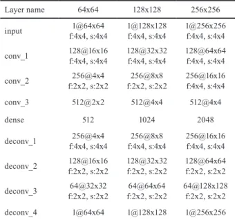
The filter and layer sizes were different for different input and output resolutions; the corresponding sizes are summarized in Table 1.

Table 1 Layer and filter sizes for different input and output resolutions.

Zero padding is not indicated, since it was 0 for each of the filters.

Layer name 64x64 128x128 256x256

input 1@64x64

f:4x4, s:4x4 1@128x128

f:4x4, s:4x4 1@256x256 f:4x4, s:4x4

conv_1 128@16x16

f:4x4, s:4x4 128@32x32

f:4x4, s:4x4 128@64x64 f:4x4, s:4x4

conv_2 256@4x4

f:2x2, s:2x2 256@8x8

f:2x2, s:2x2 256@16x16 f:4x4, s:4x4

conv_3 512@2x2 512@4x4 512@4x4

dense 512 1024 2048

deconv_1 256@4x4

f:4x4, s:4x4 256@8x8

f:4x4, s:4x4 256@16x16 f:4x4, s:4x4

deconv_2 128@16x16

f:2x2, s:2x2 128@32x32

f:2x2, s:2x2 128@64x64 f:2x2, s:2x2

deconv_3 64@32x32

f:2x2, s:2x2 64@64x64

f:2x2, s:2x2 64@128x128 f:2x2, s:2x2

deconv_4 1@64x64 1@128x128 1@256x256

Fig. 6 Topology of the convolutional neural network for an input resolution of 128 x 128. Conv and deconv stands for convolutional layer and transposed convolutional layer, respectively. Filter properties (filter size, stride, zero padding) of a layer are denoted at the preceding layer, since the filter is applied

there. Filters are depicted for the first convolutional and for the last transposed convolutional layer only. Visualization based on [17].

+ ·

sgn

input 1@128x128 f:4x4,s:4x4,z:0x0 conv1 1@32x32 f:4x4,s:4x4,z:0x0 conv2 1@8x8 f:2x2,s:2x2,z:0x0 conv3 512@4x4 ﬂatten dense 1024

deconv1 256@8x8 f:4x4,s:4x4,z:0x0 deconv2 128@32x32 f:2x2,s:2x2,z:0x0 deconv3 64@64x64 f:2x2,s:2x2,z:0x0 deconv4 1@128x128 output 1@128x128

(7)

Since this is a feed-forward neural network, the dataflow in the graph is as follows. The network takes the signed distance function on its input and processes it with three convolutional layers. The output of the last convolutional layer is flattened and fed to a densely connected layer.

Thereafter, a transposed convolutional part is coming, wherewith the velocity fields are constructed in the x and y directions, separately. Gradient information to align the weights of the network is computed by backpropagation.

There is a residual connection between the output of the first convolutional layer and the input of the second transpose convolutional layer. The connection was utilized according to the results of the hyperparameter optimization discussed in [11]. The technique itself is introduced in [18]

to overcome the vanishing gradient problem in deep neural networks and to improve convergence of such networks.

Finally, the output is multiplied by the sign function of the input to mask the out-of-domain area from the predictions. This connection was kept during inference to guarantee, that the CNN predicts non-zero elements for the velocity field only inside the fluid domain.

The weights of the network were optimized with the Adam optimizer (introduced in [19]) while the mean squared error was considered as the loss metric. As the output is field data, the point-wise loss was averaged over the fluid domain. The metrics, the neural network topology and its training were built up with TensorFlow [20].

4 Numerical experiments and results

Although the experiment was conducted to get an impres- sion on the performance of predictive initializing, the initializer had to be trained first. The details of the data generation, the training of the model and the conduction of the tests are presented in this section.

4.1 Fitting the predictive initializer

5000 different geometries were generated from the full parameter space with latin hypercube sampling [21]. The size of the dataset is in concordance roughly with the number of evaluations in an optimization session for a geometry with similar complexity (similar number of descriptive parameters) according to [1, 5].

According to Braembussche in [1] and Verstraete et al.

in [12], artificial neural networks give better predictions when they are trained on a DOE sampled dataset than trained on a random dataset which is uniformly distrib- uted. In the present experiment, the latin hypercube sampling was utilized only to guarantee that no two identical

geometries are in the original dataset, possible additional benefits were not investigated.

The corresponding flow fields were calculated thereafter with the CFD setup described above and the data for the input (signed distance field) and the output (velocity fields in the x- and in the y-direction) of the CNN. Besides, the number of the outer iteration steps of the fluid dynamics solver was measured and was written to a log file in accor- dance with the descriptive parameters of the geometry.

Data were split randomly into training, validation and test sets with a ratio of 0.8, 0.1, 0.1 compared to the size of the original set, respectively.

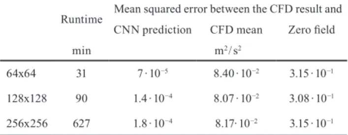
Thereafter, the three neural networks were trained with the three datasets of different resolution. The training was stopped in each case when the loss measured on the validation dataset has not been changed for 30 epochs. The hard- ware used was an NVIDIA GeForce Titan Xp GPU, the runtimes are summarized in Table 2. The mean squared error (MSE) computed on the test set and the MSE values for 2 dummy predictions (predicting the mean of the field in every grid point and predicting zero everywhere) are also indicated in the same place. The latter ones serve as baselines to obtain an idea on the quality of the result achieved with the neural network.

The result of a specific geometry from the test set is depicted in Fig. 3 where the velocity fields computed by the CFD solver and the proposed convolutional deep neural network is presented.

4.2 Performance of the predictive initializer

The trained model was utilized to give a better initial condition for the velocity field as the commonly used „everywhere zero” initial condition. The latter is referred to as cold start here, while warm start refers to the use of the predicted velocity field as an initial condition.

The data in the test database were re-evaluated with the same CFD code and setup as in the data generation phase

Table 2 Training runtimes and accuracies calculated on the equidistant grid used by the predictive initializer. The loss metric is communicated for 2 types of dummy predictions: the mean of the velocity field computed

with CFD and the zero velocity field.

Runtime Mean squared error between the CFD result and CNN prediction CFD mean Zero field

min m²/ s²

64x64 31 7 ∙ 10⁻⁵ 8.40 ∙ 10⁻² 3.15 ∙ 10⁻¹

128x128 90 1.4 ∙ 10⁻⁴ 8.07 ∙ 10⁻² 3.08 ∙ 10⁻¹ 256x256 627 1.8 ∙ 10⁻⁴ 8.17∙ 10⁻² 3.15 ∙ 10⁻¹

(8)

but with the initial velocity fields changed those predicted by the CNN. As the numerical solver starts from a condition that is closer to the real solution (as depicted in Fig. 3), a smaller runtime and a faster convergence are expected.

To conduct a CFD simulation with warm-starting (initializing the velocity fields with the predictions from the CNN), the following steps were taken.

1. The geometry was built up according to the parameter list.

2. The geometry was meshed by a meshing script.

3. The signed distance field of the fluid domain and the coordinates of the cell centers of the numerical grid were extracted.

4. The velocity fields were predicted according to the representation of the geometry, and the results were interpolated on the numerical grid.

5. New initial conditions were written for the numerical solver; the computation was executed.

6. The number of the outer steps taken by the numerical solver was written to a database.

The time required for the predictions was not considered here, since it was several magnitudes less than the time-requirement of the CFD simulations [11].

The steps above were conducted on every element of the test data set. Thereafter, the speedup of the simulation was calculated as the ratio of the number of iteration steps with cold start and the number of iteration steps with warm start.

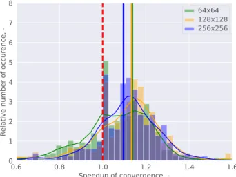
Preliminary results are depicted in Fig. 7. The speedup is summarized in the histogram for the test dataset and for the three different resolutions. The y-axis is normalized, the area under the bars for a specific resolution sums up to 1.

Although some speedup is seen in the convergence of the simulation, the results are not satisfying. The poor performance of the network with the finest resolution was unexpected, thus further examination was conducted.

By checking the geometries with the worst speedup (with a decrease in convergence speed), it has been found, that the predictive initializer sometimes predicts non-zero wall velocities. This leads to the form of high-velocity, artificial flow structures during the iterative steps of the CFD simulator but these structures vanish later on.

To overcome this adverse effect, a second experiment was conducted, where the predicted velocity was multiplied by a factor of 0.25 in the cells adjacent to the wall.

The results are depicted in Fig. 8.

The highest speedup belongs to the finest resolution, though the mean calculated on the full test set is just

slightly higher than the best one in the previous case. This is unexpected in the light of Fig. 3.

The explanation comes from the different resolutions of the grids used for the prediction and for the numerical simulation. As the finest resolution grid wherein the velocity field gets predicted is still coarse compared to the numerical mesh, Fig. 3. presents the bulk flow only.

The boundary layer is thinner than the resolution of the predicted output, so, the near-wall treatment has an effect

Fig. 7 Speedup of the convergence with warm starting the simulations with three different resolution velocity field. The y-axis is normalized, thus the area under the bars for a specific resolution sums up to 1. Bars over 1.0 mean acceleration in convergence speed. The mean for each

network is denoted by a vertical line.

Fig. 8 Speedup of the convergence with warm starting the simulations with three different resolution velocity field. The y-axis is normalized, thus the area under the bars for a specific resolution sums up to 1.

Bars over 1.0 mean acceleration in convergence speed. The mean for each network is denoted by a vertical line. The predicted velocity was

multiplied by a factor of 0.25 in the near-wall cells.

(9)

References

[1] Thévenin, D., Janiga, G. "Optimization and Computational Fluid Dynamics", 1st ed., Springer-Verlag Berlin Heidelberg, Berlin, Germany, 2008.

https://doi.org/10.1007/978-3-540-72153-6

[2] Skinner, S. N., Zare-Behtash, H. "State-of-the-art in aerodynamic shape optimisation methods", Applied Soft Computing, 62, pp. 933–962, 2018.

https://doi.org/10.1016/j.asoc.2017.09.030

[3] Sacks, J., Welch, W. J., Mitchell, T. J., Wynn, H. P. "Design and Analysis of Computer Experiments", Statistical Science, 4(4), pp. 409–423, 1989.

https://doi.org/10.1214/ss/1177012413

[4] Krige, D. G. "A Statistical Approach to Some Basic Mine Valuation Problems on the Witwatersrand", Journal of the Chemical, Metallurgical and Mining Society of South Africa, 52(6), pp.

119–139, 1951. [online] Available at: https://journals.co.za/content/

saimm/52/6/AJA0038223X_4792 [Accessed: 20 February 2019]

[5] Booker, A. J., Dennis, J. E., Frank, P. D., Serafini B. D., Torczon V., Trosset M. W. "A rigorous framework for optimization of expen- sive functions by surrogates", Structural Optimization, 17(1), pp. 1–13, 1999.

https://doi.org/10.1007/BF01197708

[6] Simpson, T. W., Poplinski, J., Koch, P. N., Allen, J. K. "Metamodels for Computer-based Engineering Design: Survey and recommen- dations", Engineering with Computers, 17(2), pp. 129–150, 2001.

https://doi.org/10.1007/PL00007198

[7] Simpson, T. W., Booker, A. J., Ghosh, D., Giunta, A. A., Koch, P. N., Yang, R.-J. "Approximation methods in multidisciplinary analysis and optimization: a panel discussion", Structural and Multidisciplinary Optimization, 27(5), pp. 302–313, 2004.

https://doi.org/10.1007/s00158-004-0389-9

[8] Simpson, T. W., Toropov, V., Balabanov, V., Viana, F. A. C. "Design and Analysis of Computer Experiments in Multidisciplinary Design Optimization: A Review of How Far We Have Come - Or Not", In:

12th AIAA/ISSMO Multidisciplinary Analysis and Optimization Conference, Victoria, British Columbia, Canada, 2008, pp. 1–22.

https://doi.org/10.2514/6.2008-5802

[9] Weinmeister, J., Gao, X., Roy, S. "Analysis of a Polynomial Chaos-Kriging Metamodel for Uncertainty Quantification in Aerodynamics", AIAA Journal, Ahead of printing, pp. 1–17, 2019.

https://doi.org/10.2514/1.J057527

[10] Li, L., Cheng, Z., Lange, C. F. "CFD-Based Optimization of Fluid Flow Product Aided by Artificial Intelligence and Design Space Validation", Mathematical Problems in Engineering, 2018, pp. 1–14, 2018.

https://doi.org/10.1155/2018/8465020

[11] Hajgató, G., Gyires-Tóth, B., Paál, G. "Predicting the flow field in a U-bend with deep neural networks", In: Proceedings of Conference on Modelling Fluid Flow (CMFF’18): 17th event of the International Conference Series on Fluid Flow Technologies, Budapest, Hungary, 2018, pp. 1–8.

outside the boundary layer as well. This leads to an arti- ficially thicker boundary layer in the prediction than in the real case, and it takes a lot of iterations to wash it out from the domain.

5 Conclusions and outlook

Predictive initialization has been presented here, wherewith aerodynamic shape optimization can be accelerated.

The CFD simulation of 500 different U-bend shapes was initialized with the novel technique, wherewith a mean speedup of 13 % was achieved without any loss in accuracy.

The initializer can be trained on the results of a preliminary optimization session (which is common in practice) or on a dataset generated specifically to train the neural network. Thereafter, the optimization can be carried out with an extended framework like the one depicted in Fig. 2.

At the present state, only a significantly smaller speedup can be achieved by the predictive initializer proposed in this paper compared to using conventional metamodels but where accuracy is a must, metamodels cannot be utilized. This is more straightforward by looking at the

conceptual differences depicted in Fig. 1. (for metamodels) and Fig. 2 (for predictive initialization).

In addition, the predictive initializer presented here does not depend on the descriptive parameters of the geometry, so, if a similar geometry is optimized with another parameterization, the initializer can be re-used without re- training. This is even true for such cases, where the new geometries have small areas lying outside the range of the training geometries according to [11].

Moreover, better results are expected to be achieved with the further development in the handling of the near- wall cell velocities.

Acknowledgement

The research presented in this paper has been sup- ported by the BME-Artificial Intelligence FIKP grant of Ministry of Human Resources (BME FIKP-MI/SC) and by János Bolyai Research Scholarship of the Hungarian Academy of Sciences. We gratefully acknowledge the support of NVIDIA Corporation with the donation of the Titan Xp GPU used for this research.

(10)

[12] Vertsraete, T., Coletti, F., Bulle, J., Vanderwielen, T., Arts, T.

"Optimization of a U-Bend for Minimal Pressure Loss in Internal Cooling Channels: Part I—Numerical Method", In: ASME 2011 Turbo Expo: Turbine Technical Conference and Exposition, Vancouver, British Columbia, Canada, 2011, pp. 1665–1676.

https://doi.org/10.1115/GT2011-46541

[13] Geuziane, C., Remacle, J-F. "Gmsh: a 3-D finite element mesh generator with built-in pre- and post-processing facilities", International Journal for Numerical Methods in Engineering, 79, pp. 1309–1331, 2009.

https://doi.org/10.1002/nme.2579

[14] Weller, H. G., Tabor, G., Jasak, H., Fureby, C. "A tensorial approach to computational continuum mechanics using object-oriented techniques", Computers in Physics, 12(6), pp. 620–631, 1998.

https://doi.org/10.1063/1.168744

[15] Ferziger, J. H., Perić, M. "Computational Methods for Fluid Dynamics", 3rd ed., Springer-Verlag Berlin Heidelberg, Berlin, Germany, 2002.

https://doi.org/10.1007/978-3-642-56026-2

[16] Guo, X., Li, W., Iorio, F. "Convolutional Neural Networks for Steady Flow Approximation", In: Proceedings of the 22nd ACM SIGKDD International Conference on Knowledge Discovery and Data Mining, San Francisco, California, USA, 2016, pp. 481–490.

https://doi.org/10.1145/2939672.2939738

[17] Iqbal, H. "PlotNeuralNet", [computer program] Available at:

https://doi.org/10.5281/zenodo.2526396

[18] He, K., Zhang, X., Ren, S., Sun, J. "Deep Residual Learning for Image Recognition", In: 2016 IEEE Conference on Computer Vision and Pattern Recognition, Las Vegas, Nevada, USA, 2016, pp. 770–778.

https://doi.org/10.1109/CVPR.2016.90

[19] Kingma, D. P., Ba, L. J. "Adam: A Method for Stochastic Optimization", In: International Conference on Learning and Representations, San Diego, California, USA, 2015, pp. 1–13.

[online] Available at: https://arxiv.org/abs/1412.6980v5 [Accessed:

20 February 2019]

[20] Abadi, M., Agarwal, A., Barham, P., Brevdo, E., Chen, Z., Citro, C., Corrado, G. S., Davis, A., Dean, J., Devin, M., Ghemawat, S., Goodfellow, I., Harp, A., Irving, G., Isard, M., Jozefowicz, R., Jia, Y., Kaiser, L., Kudlur, M., Levenberg, J., Mané, D., Schuster, M., Monga, R., Moore, S., Murray, D., Olah, C., Shlens, J., Steiner, B., Sutskever, I., Talwar, K., Tucker, P., Vanhoucke, V., Vasudevan, V., Viégas, F., Vinyals, O., Warden, P., Wattenberg, M., Wicke, M., Yu, Y., Zheng, X. "TensorFlow: Large-scale machine learning on heterogeneous systems", [computer program] Available at: https://

www.tensorflow.org

[21] McKay, M. D., Beckman, R. J., Conover, W. J. "A Comparison of Three Methods for Selecting Values of Input Variables in the Analysis of Output from a Computer Code", Technometrics, 21(2), pp. 239–245, 1979.

https://doi.org/10.2307/1268522