Maintainability of classes in terms of bug prediction

(1)

Maintainability of classes in terms of bug prediction

Gergely Ladányi

University of Szeged Department of Software Engineering

Hungary

lgergely@inf.u-szeged.hu

Submitted October 27, 2015 — Accepted April 18, 2016

Abstract

Measuring software product maintainability is a central issue in software engineering which led to a number of different practical quality models. Be- sides system level assessments it is also desirable that these models provide technical quality information at source code element level (e.g. classes, methods) to aid the improvement of the software. Although many existing models give an ordered list of source code elements that should be improved, it is unclear how these elements are affected by other important quality indicators of the system, e.g. bug density.

In this paper we empirically investigate the bug prediction capabilities of the class level maintainability measures of our ColumbusQM probabilistic quality model using open-access PROMSIE bug dataset. We show that in terms of correctness and completeness, ColumbusQM competes with statistical and machine learning prediction models especially trained on the bug data using product metrics as predictors. This is a great achievement in the light of that our model needs no training and its purpose is different (e.g. to estimate testability, or development costs) than those of the bug prediction models.

Keywords: ISO/IEC 25010, ColumbusQM, Software maintainability, Bug, Bug prediction, Class level maintainability, PROMISE

http://ami.ektf.hu

121

(2)

1. Introduction

Maintainability is probably one of the most attractive, observed and evaluated quality characteristics of software products. The importance of maintainability lies in its direct connection with many factors that influence the overall costs of a software system, for example the effort needed for new developments [1], mean time between failures of the system [2], bug fixing time [3], or operational costs [4]. After the appearance of the ISO/IEC 9126 standard [5] for software product quality, the development of new practical models which measure the maintainability of systems in a direct way has exploded [6, 7, 8, 9, 10].

Although these models provide a system level overview about the maintainability of a software which is a valuable information in itself for e.g. making decisions, backing up intuition, or assessing risks, just a portion of them provide low-level, actionable information for developers (i.e. list of source code elements and quality attributes that should be improved). Current approaches usually just enumerate the most complex methods, most coupled classes or other source code elements that carry some source code metric value. There is a lack of empirical evidences that these elements are indeed the most critical from maintainability point of view and changing them will improve some of the quality factors related to maintainability.

We used our earlier results to calculate maintainability on system and lower levels. The ColumbusQM model introduced in our previous work [10] is able to calculate maintainability on systems level. Later we extended the ColumbusQM with the drill-down approach [11] to calculate maintainability on lower levels as well (classes, methods, etc.). The drill-down approach calculates a so-called relative maintainability index (RMI) for each source code element which measures the extent to which they affect the overall system maintainability. The RMI is a small number that is either positive when it improves the overall rating or negative when it decreases the system level maintainability. We also developed a web based graphical user interface called QualityGate [12] to continuously monitor the maintainability of a software using version control systems.

The contribution of this study is the comparison of the RMI based ordering of classes with widely used statistical and machine learning prediction models, e.g. decision trees, neural networks, or regression. The performance of the RMI based ordering of classes proves to be competitive compared to these prediction techniques.

The paper is organized as follows. Section 2 presents the work related to ours.

The data collection and analysis methodology is introduced in Section 3, while the analysis results are described in Section 4. Finally, we list the threats to validity in Section 5, and conclude the paper in Section 6.

2. Related work

In this section will give an overview about the related papers dealing with software quality measurement and fault prediction.

(3)

Both of software fault detection [13, 14] and software quality models [15, 16]

date back to the 70’s and evolving since then [17, 18]. Although the software quality measurement has become popular recently by the release of quality standards like ISO/IEC 9126 [5] and its successor the ISO/IEC 25010 [19]. Using the definition of the characteristics and subcharacteristics reseachers developed several software quality models which are able to measure the software quality of a system, but only a few works on lower class or method level. Even fewer works investigate empirically the relation of the maintainability and other factors, like bug density at finer levels.

Heitlager et al. [6] presented a bottom-up approach to measure software maintainability. They split the basic metric values into five categories from poor to excellent using threshold values [20]. Then they aggregated these qualifications for for higher properties, such as maintainability. Bijlsma et al. [21] examined the correlation of the SIG model rating with four maintainability related factors: Time, Throughput, Productivity, Efficiency. They found that their model has a strong predictive power for the maintenance burden that is associated to the system. Our maintainability model is in many aspects similar to the SIG model; however, we use a probabilistic approach for aggregation opposed to the threshold based approach, and also generate a list of source code elements with the highest risk that should be improved first. Moreover, we investigate the relation of maintainability and bugs at lower level rather than system level where immediate actions can be taken.

The technical debt based models like SQALE [8] or SQUALE [7] introduce low- level rules to connect the ISO/IEC 9126 characteristics with metrics. These rules refer to different properties of the source code (e.g. the comment ratio should be above 25%) and violating them has a reparation cost. These models provide a list of critical elements simply by ordering them based on their total reparation costs.

Although it assures the biggest system level maintainability increase there is no guarantee that one corrects the most critical elements (e.g. elements with the most bugs, or elements that are used by many other components).

Chulani et. al. [22] introduced the Orthogonal Defect Classification Construc- tive Quality Model (ODC COQUALMO) as an extension of the Constructive Cost Model (COCOMO) [23, 24]. The model was calibrated with empirical defect dis- tributions and it contains two sub-models. Defect introduction sub-model predicts the number of defects that will appear in each defect category. The defect removal model produces an estimate of the number of defects that will be removed from these categories. The idea behind this and our study is similar, the main difference is that we did not add a bug predictor sub-model to our quality model but we investigated the connection between the defects and the final aggregated value of the model.

Chawla [25] proposed the SQMMA (Software Quality Model for Maintainability Analysis) approach based on the ISO/IEC 25010 standard which provides compre- hensive formulas to calculate the Maintainablity and its subcharacteristic. They normalized the average metric values respect to the first selected release of Tomcat and they aggregated towards higer nodes using weighted sum. They also compared

(4)

the number of buggy files with the system-level quality measurements through four versions of the Tomcat. They observed that the pattern of Maintainability consis- tently matches (in reverse) with the number of buggy files in the system. We also compared the maintainability with the bugs in a system, but we worked on the level of classes instead of the system.

Papers related to software defects very often use databases with information about bugs and different metrics about the source code elements. Zimmermann et al. [26] has published a bug database for Eclipse and used the data for predicting defects by logistic regression and complexity metrics. Moser et al. [27] annotated this dataset with change metrics and compared its bug prediction ability with code metrics. We also used code metrics and a bug database, but we examined the connection between the number of bugs and the RMI value of classes rather than source code metrics directly. Moreover, the bug dataset used by Moser has become part of the PROMISE [28] database, but we could not consider these data as it provides bug information only for packages and Java files, while we need bug data on the level of classes.

Jureczko et al. [29] describes an analysis that was conducted on newly collected repository with 92 versions of 38 proprietary, open-source and academic projects.

The dataset is part of the PROMISE dataset and part of the our study as well since it provides bug information on class level. To study the problem of cross project defect prediction they performed clustering on software projects in order to identify groups of software projects with similar characteristic from the defect prediction point of view. The conducted analysis reveals that there exist clusters from the defect prediction point of view, and two of those clusters were successfully identified. Later Madeyski et al. [30] used the dataset to empirically investigate how process metrics can significantly improve defect prediction.

There are also other works relying on the PROMISE dataset. Menzies et al.

aim to comparatively evaluate local versus global lessons learned [31] for effort estimation and defect prediction. They applied automated clustering tools to effort and defect datasets from the PROMISE repository and rule learners generated lessons learned from all the data. The work of Wang and Yao [32] deals with improving the bug prediction models by handling imbalanced training data and uses PROMISE dataset to validate the approach.

Vasilescu et. al. [33] aggregated the SLOC class level metric to package level using various aggregation techniques (Theil, Gini, Kolm, Atkinson, indices, sum, mean, median). They found that the choice of the aggregation technique does influence the correlation of the aggregated values and the number of defects. Con- trary to them we did not aggregate class level metrics to package level metrics, but we aggregated them to a maintainability index using the ColumbusQM quality model weighed by experts and compared the results with the number of bugs in the classes.

(5)

3. Methodology

We started the empirical examination of the bugs in the aspects of maintainability by collecting bug datasets. In the literature the most widely used bug dataset is the PROMISE dataset [34]. It contains bug information on class level for various open-source and proprietary systems. Since for the maintainability calculation the source code is necessary we only used the open-source systems from the dataset.

In order to decrease the possible bias in the machine learning prediction models we filter out the very small systems (i.e. systems with fewer than 6 classes) and those having very high ratio of buggy classes (i.e. over 75% of the classes contain bugs). At the end of the process we collected source code and bug information for each 30 versions of the 16 open-source systems. For each Java class found in these 30 versions we calculate the class level RMI value (relative maintainability index) according to our drill-down approach [11].

3.1. The applied quality model

First we calculated the absolute maintainability values for the different versions of the systems. We used the ColumbusQM, our probabilistic software quality model [10] that is able to measure the quality characteristics defined by the ISO/IEC 25010 standard. The computation of the high-level quality characteristics is based on a directed acyclic graph (see Figure 1) whose nodes correspond to quality properties that can either be internal (low-level) or external (high-level).

Internal quality properties characterize the software product from an internal (de- veloper) view and are usually estimated by using source code metrics. External quality properties characterize the software product from an external (end user) view and are usually aggregated somehow by using internal and other external quality properties. The nodes representing internal quality properties are called sensor nodes as they measure internal quality directly (white nodes in Figure 1).

The other nodes are calledaggregate nodesas they acquire their measures through aggregation of the lower-level nodes. In addition to the aggregate nodes defined by the standard (black nodes) we introduced new ones (light gray nodes) and kept those of contained only in the old standard (dark gray nodes).

The description of the different quality attributes can be found in Table 1.

Dependencies between an internal and an external, or two external properties are represent by the edges of the graph. The aim is to evaluate all the external quality properties by performing an aggregation along the edges of the graph, called Attribute Dependency Graph (ADG). We calculate a so calledgoodness value(from the [0,1] interval) to each node in the ADG that expresses how good or bad (1 is the best) is the system regarding that quality attribute. The probabilistic statistical aggregation algorithm uses a benchmark as the basis of the qualification, which is a source code metric repository database with 100 open-source and industrial software systems.

(6)

Figure 1: ColumbusQM – Java ADG [35]

3.2. The drill-down approach

The above approach is used to obtain a system-level measure for source code maintainability. Our aim is to drill down to lower levels in the source code and to get a similar measure for the building blocks of the code base (e.g. classes or methods). For this, we defined therelative maintainability index¹ (RMI)for the source code elements [11], which measures the extent to which they affect the system level goodness values. The basic idea is to calculate the system level goodness values, leaving out the source code elements one-by-one. After a particular source code element is left out, the system level goodness values will change slightly for each node in the ADG. The difference between the original goodness value computed for the whole system and the goodness value computed without the particular source code element is called therelative maintainability indexof the source code element itself. The RMI is a small number that is either positive when it improves the overall rating or negative when it decreases the system level maintainability. The absolute value of the index measures the extent of the influence to the overall system level maintainability. In addition, a relative index can be computed for each node of the ADG, meaning that source code elements can affect various quality aspects in different ways and to different extents.

More details and the validation of the approach can be found in our previous paper [11].

3.3. Comparison of ColumbusQM and prediction models

One way to look at the maintainability scores is that they rank classes according to their level of maintainability. Nonetheless, if we assume that classes with the worst maintainability scores contain most of the bugs we can easily turn RMI into

1We use the terms relative maintainability index, relative maintainability score, and RMI interchangeably throughout the paper. Moreover, we may also refer to them by omitting the word “relative” for simplicity reasons.

(7)

Table 1: The low-level quality properties of our model [35]

Sensor nodes

CC Clone coverage. The percentage of copied and pasted source code parts, computed for the classes of the system.

NOA Number of Ancestors. Number of classes, interfaces, enums and annotations from which the class is directly or indirectly inherited.

WarningP1 The number of critical rule violations in the class.

WarningP2 The number of major rule violations in the class.

WarningP3 The number of minor rule violations in the class.

AD Api Documentation. Ratio of the number of documented public methods in the class.

CLOC Comment Lines of Code. Number of comment and documentation code lines of the class.

CD Comment Density. The ratio of comment lines compared to the sum of its comment and logical lines of code.

TLOC Total Lines of Code. Number of code lines of the class, including empty and comment lines.

NA Number of attributes in the class.

WMC Weighted Methods per Class. Complexity of the class expressed as the number of linearly independent control flow paths in it. It is calculated as the sum of the McCabe’s Cyclomatic Complexity (McCC) values of its local methods and init blocks.

NLE Nesting Level Else-If. Complexity of the class expressed as the depth of the maximum embeddedness of its conditional and iteration block scopes, where in the if-else-if construct only the first if instruction is considered.

NII Number of Incoming Invocations. Number of other methods and attribute initializations, which directly call the local methods of the class.

RFC Response set For Class. Number of local (i.e. not inherited) methods in the class plus the number of directly invoked other methods by its methods or attribute initializations.

TNLM Total Number of Local Methods. Number of local (i.e. not inherited) methods in the class, including the local methods of its nested, anonymous, and local classes.

CBO Coupling Between Object classes. Number of directly used other classes (e.g.

by inheritance, function call, type reference, attribute reference).

a simple classification method. For that we should define “classes with the worst maintainability scores” more precisely. To be able to compare the RMI based classification to other prediction models, we simply use the natural RMI threshold of 0, i.e. our simple model classifies all the classes as buggy which have negative maintainability scores, and non-buggy all the rest.

Now we are ready to compare the ColumbusQM based ordering (i.e. classification with the above extension) to other well-known statistical and machine learning prediction models. We examine two types of models, three classification methods:

J48 decision tree algorithm, neural network model, and a logistic regression based algorithm. Additionally, we apply three regression techniques that differ from the above classifiers in that they assign a real number (the predicted number of bugs in the class) to each class instead of predicting only whether it is buggy or not. We consider the RepTree decision tree based regression algorithm, linear regression,

(8)

and neural network based regression. In case of regression algorithms we say that the algorithm predicts a class as buggy if it predicts more than 0.5 bugs for it, because above this number the class will more likely be buggy than not buggy.

These models need a training phase to build a model for prediction. We chose to put all the classes from the different versions of the systems together and train these algorithms on this huge dataset using 10-fold cross validation. We allow them to use all the available source code metrics which the Columbus static analyzer tool calledSourceMeter provides – not only those used by ColumbusQM – as predictors.

After the training we run the prediction on each of the 30 separate versions of the 13 systems. For building the prediction models we use the Weka tool [36].

We used Spearman’s rank correlation coefficient to measure the strength of the similarity between the orderings of machine learning models and RMI. We also evaluate the performance of the prediction models and our maintainability model in terms of the classical measures of precision and recall. In addition, we also calculate thecompleteness value [37], which measures the number of bugs (faults) in classes classified fault-prone, divided by the total number of faults in the system.

This number differs from the usual recall value as it measures the percentage of faults – and not only the faulty classes – that has been found by the prediction model.

Each model predicts classes as either fault-prone or not fault-prone, so the classification is binary (in case of regression models we make the prediction binary as described above). The definition of the performance measures used in this work are as follows:

Precision:=# classes correctly classified as buggy

# total classes classified as buggy Recall:=# classes correctly classified as buggy

# total buggy classes in the system Completeness:=# bugs in classes classified buggy

# total bugs in the system

To be able to directly compare the results of different models we also calculate the F-measure, which is the harmonic mean of precision and recall:

F−measure:= 2· precision·recall precision+recall

As an additional aggregate measure we define the F˙-measure to be the harmonic mean of precision and completeness:

F˙ −measure:= 2· precision·completeness precision+completeness

(9)

4. Results

The empirical analysis is performed on 30 releases of 13 different open-source systems that take up to 2M lines of source code. The bug data for these systems is available in the PROMISE [28] online bug repository which we used for collecting the bug numbers at class level. For each version of the subject systems we calculated the system level quality according to Section 3.1 and all the relative maintainability scores for classes as described in Section 3.2 using ColumbusQM [10].

Table 2: Descriptive statistics of the analyzed systems [35]

System Nr. of Nr. of Buggy

classes bugs classes

ant-1.3 115 33 20

ant-1.4 163 45 38

ant-1.5 266 35 32

ant-1.6 319 183 91

ant-1.7 681 337 165

camel-1.0 295 11 10

camel-1.2 506 484 191

camel-1.4 724 312 134

camel-1.6 795 440 170

ivy-1.4 209 17 15

ivy-2.0 294 53 37

jedit-3.2 255 380 89

jedit-4.0 288 226 75

jedit-4.1 295 215 78

jedit-4.2 344 106 48

jedit-4.3 439 12 11

log4j-1.0 118 60 33

log4j-1.1 100 84 35

lucene-2.0 180 261 87

pbeans-2.0 37 16 8

poi-2.0 289 39 37

synapse-1.0 139 20 15

synapse-1.1 197 96 57

synapse-1.2 228 143 84

tomcat-6.0 732 114 77

velocity-1.6 189 161 66

xalan-2.4 634 154 108

xalan-2.6 816 605 395

xerces-1.2 291 61 43

xerces-1.3 302 186 65

Average 341.33 162.97 77.13

Table 2 shows some basic descriptive statistics about the analyzed systems. The second column contains the total number of classes in the systems (that we could

(10)

successfully map) while the third column shows the total number of bugs. The fourth column presents the number of classes containing at least one bug.

4.1. Prediction Model Results

Recall, that to compare our model to other prediction models we put all the classes together and let the machine learning algorithms to build prediction models based on all the available product metrics using 10-fold cross validation. We built three binary classifiers based on J48 decision tree, logistic regression, and neural network;

and three regression based prediction models using RepTree decision tree, linear regression, and neural network.

Classification algorithms. First, we present the results of the comparison of classifiers and maintainability score. For each of the classifiers we ran the classification on the classes of the 30 versions of the subject systems. As described in Section 3, we also classified the same classes based on our maintainability scores.

Finally, we calculated the precision, recall, and completeness measures (for the definitions of these measures see Section 3) for the different predictions for each subject system.

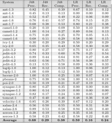
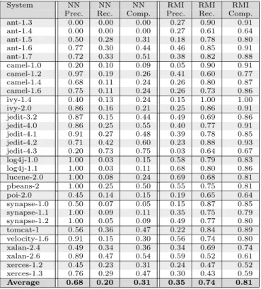
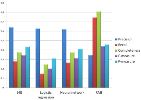
Table 3 and 4 lists all the precision, recall, and completeness values for the four different methods and for all the 30 versions of the 13 subject systems. Although the results are varying for the different systems, in general we can say that the precisions of the three learning based models are higher than that of the RMI based model. The average precision values are 0.68, 0.59, 0.68, and 0.35 for J48, logistic regression (LR), neural network (NN), and RMI, respectively. Nonetheless, in terms of recall and completeness especially, RMI looks superior to the other methods.

The average completeness values are 0.38, 0.24, 0.31, and 0.81 for J48, logistic regression, neural network, and RMI, respectively. Figure 2 shows these values on a bar-chart together with the F-measure (harmonic mean of the precision and recall) andF˙-measure (harmonic mean of the precision and completeness values).

It is easy to see that according to both the F-measure and F-measure, RMI and˙ J48 methods are performing the best. But while J48 achieves this with very high precision and an average recall and completeness, RMI has far the highest recall and completeness values combined with moderate precision. Another important observation is that for every method the average recall values are smaller than the completeness values which suggests that the bug distribution among the classes of the projects is fairly uniform.

RMI performs the worst (in terms of precision) in cases ofcamel v1.0 andjedit v4.3. Exactly these two systems are those where the number of bugs per class are the smallest (11/295 and 12/439 respectively). This biases not only our method but the other algorithms, too. They achieve the lowest precision on these two systems.

There is a block of precision values close to 1 for systems from log4j v1.0 to pbeans v2.0 for the three learning based models. However, their completeness measure is very low (and recall is even lower). On the contrary, RMI has a very

(11)

Table 3: Comparison of the precision, recall, and completeness of different models

System J48 J48 J48 LR LR LR

Prec. Rec. Comp. Prec. Rec. Comp.

ant-1.3 0.82 0.45 0.39 0.67 0.10 0.12

ant-1.4 0.45 0.13 0.13 0.00 0.00 0.00

ant-1.5 0.52 0.47 0.49 0.22 0.06 0.09

ant-1.6 0.76 0.41 0.57 0.74 0.15 0.25

ant-1.7 0.68 0.38 0.53 0.80 0.21 0.38

camel-1.0 0.20 0.10 0.09 0.50 0.10 0.09

camel-1.2 1.00 0.14 0.27 0.89 0.04 0.13

camel-1.4 0.75 0.20 0.25 0.70 0.05 0.15

camel-1.6 0.68 0.11 0.29 0.58 0.06 0.15

ivy-1.4 0.30 0.20 0.29 0.50 0.20 0.29

ivy-2.0 0.65 0.35 0.43 0.58 0.30 0.38

jedit-3.2 0.80 0.27 0.57 0.75 0.17 0.45

jedit-4.0 0.74 0.33 0.60 0.76 0.25 0.54

jedit-4.1 0.89 0.44 0.64 0.91 0.27 0.48

jedit-4.2 0.63 0.56 0.71 0.56 0.38 0.57

jedit-4.3 0.13 0.55 0.58 0.09 0.36 0.33

log4j-1.0 1.00 0.12 0.13 1.00 0.06 0.07

log4j-1.1 1.00 0.09 0.12 0.50 0.03 0.07

lucene-2.0 1.00 0.15 0.25 1.00 0.07 0.18

pbeans-2 0.75 0.38 0.56 1.00 0.13 0.19

poi-2.0 0.50 0.19 0.21 0.47 0.19 0.21

synapse-1.0 0.80 0.27 0.35 0.00 0.00 0.00

synapse-1.1 0.80 0.14 0.19 0.00 0.00 0.00

synapse-1.2 0.82 0.17 0.24 1.00 0.05 0.07

tomcat-1 0.47 0.40 0.46 0.48 0.36 0.48

velocity-1.6 0.85 0.26 0.39 0.67 0.12 0.20

xalan-2.4 0.56 0.50 0.55 0.50 0.31 0.38

xalan-2.6 0.89 0.53 0.58 0.94 0.33 0.40

xerces-1.2 0.38 0.19 0.25 0.35 0.16 0.23

xerces-1.3 0.58 0.23 0.42 0.58 0.22 0.40

Average 0.68 0.29 0.38 0.59 0.16 0.24

high recall and completeness in these cases (over 0.79 and 0.83, respectively) and still having acceptably high precision values (above 0.5).

Forsynapse v1.0 andv1.1 logistic regression and forant v1.3 andv1.4 neural network achieves 0 precision, recall and completeness. Again, RMI based prediction achieves a very high completeness and recall with a moderate, but still acceptable level of precision in these cases, too.

We note again, that while our maintainability model uses only 16 metrics we let the learning algorithms to use all the 59 available product metrics which we calculated. If we restricted the set of predictors for the classifier algorithms to only those that ColumbusQM uses, we got somewhat different results. Figure 3 shows the average values of the resulting precision, recall, completeness, F-measure, and F˙-measure. In this case, the precision of the learning algorithms dropped a bit while recall and completeness levels remained. The F-measure of the RMI is higher than that of any other method while in terms of F˙-measure J48 and RMI perform the best.

We empirically investigated that RMI competes with the classification based algorithms. With Spearman’s rank correlation we measured the strength of the similarity between the oredering of the RMI and the machine learning models.

(12)

Table 4: Comparison of the precision, recall, and completeness of different models

System NN NN NN RMI RMI RMI

ant-1.3 0.00 0.00 0.00 0.27 0.90 0.91

ant-1.4 0.00 0.00 0.00 0.27 0.61 0.64

ant-1.5 0.50 0.28 0.31 0.18 0.78 0.80

ant-1.6 0.77 0.30 0.44 0.46 0.85 0.91

ant-1.7 0.72 0.33 0.51 0.38 0.82 0.88

camel-1.0 0.20 0.10 0.09 0.05 0.90 0.91

camel-1.2 0.97 0.19 0.26 0.41 0.60 0.77

camel-1.4 0.68 0.11 0.24 0.26 0.80 0.87

camel-1.6 0.75 0.11 0.24 0.26 0.73 0.86

ivy-1.4 0.40 0.13 0.24 0.15 1.00 1.00

ivy-2.0 0.86 0.16 0.21 0.25 0.86 0.91

jedit-3.2 0.87 0.15 0.44 0.49 0.69 0.86

jedit-4.0 0.86 0.25 0.55 0.40 0.77 0.91

jedit-4.1 0.91 0.27 0.48 0.39 0.78 0.85

jedit-4.2 0.71 0.42 0.60 0.23 0.88 0.93

jedit-4.3 0.20 0.73 0.75 0.03 0.64 0.67

log4j-1.0 1.00 0.03 0.15 0.58 0.79 0.83

log4j-1.1 1.00 0.03 0.11 0.68 0.80 0.86

lucene-2.0 1.00 0.08 0.24 0.69 0.68 0.81

pbeans-2 1.00 0.25 0.50 0.55 0.75 0.81

poi-2.0 0.45 0.14 0.15 0.19 0.65 0.64

synapse-1.0 0.50 0.07 0.05 0.15 0.87 0.85

synapse-1.1 1.00 0.09 0.11 0.35 0.75 0.79

synapse-1.2 1.00 0.05 0.09 0.49 0.77 0.80

tomcat-1 0.56 0.36 0.47 0.22 0.84 0.89

velocity-1.6 0.91 0.15 0.30 0.56 0.74 0.80

xalan-2.4 0.49 0.34 0.36 0.34 0.69 0.74

xalan-2.6 0.89 0.47 0.54 0.59 0.52 0.61

xerces-1.2 0.45 0.23 0.31 0.24 0.47 0.52

xerces-1.3 0.76 0.29 0.47 0.30 0.43 0.59

Average 0.68 0.20 0.31 0.35 0.74 0.81

The measurements for the classication algorithms are in Table 5. If the machine learning models used only the quality model metrics the correlation in average is strong (0.669) for the Logistic Regression and moderately strong for the J48 (0.504) and the Neural Network (0.463). As it was expected if the machine learning models were able to use other metrics the correlation became lower because of the difference between the used metrics.

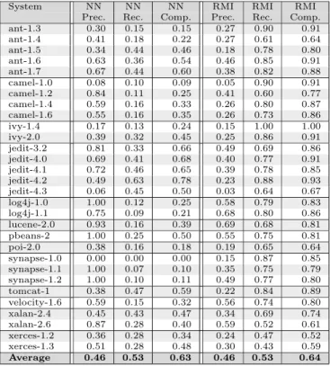
Regression based algorithms. Next, we analyze the comparison results of the regression based algorithms and RMI. Recall, that regression algorithms provide a continuous function for predicting the number of bugs instead of only classifying classes as buggy or non-buggy. According to the method described in Section 3, we consider a class as buggy in this case if the appropriate regression model predicts at least 0.5 bugs for it. The detailed results of the precision, recall, and completeness values are shown in Table 6 and 7.

In this case the overall picture is somewhat different. The regression based methods work more similarly to RMI meaning that they achieve higher recall and completeness in return for lower precision. This can also be observed in Figure 4.

All the bars on the chart are similarly distributed as in case of RMI. Neural network

(13)

Figure 2: Average performance of methods using all metrics

Figure 3: Average performance of methods using only the 16 metrics used by ColumbusQM

(14)

Table 5: Spearman’s rank correlation between the ranking of RMI and the classification algorithms

System Only QM All

J48 LR NN J48 LR NN

ant-1.3.csv 0.503 0.687 0.587 0.252 0.361 0.241 ant-1.4.csv 0.409 0.544 0.428 0.192 0.215 0.084 ant-1.5.csv 0.553 0.699 0.566 0.348 0.421 0.166

ant-1.6.csv 0.541 0.71 0.577 0.334 0.376 0.118

ant-1.7.csv 0.622 0.82 0.641 0.359 0.515 0.253

camel-1.0.csv 0.56 0.75 0.369 0.177 0.298 0.12

camel-1.2.csv 0.521 0.753 0.411 0.258 0.425 0.107 camel-1.4.csv 0.588 0.821 0.42 0.316 0.482 0.147 camel-1.6.csv 0.607 0.864 0.446 0.176 0.552 0.222 ivy-1.4.csv 0.517 0.666 0.474 0.326 0.435 0.276 ivy-2.0.csv 0.507 0.624 0.479 0.349 0.425 0.311 jedit-3.2.csv 0.194 0.239 0.035 0.131 0.077 0.102 jedit-4.0.csv 0.343 0.437 0.207 0.277 0.27 0.267 jedit-4.1.csv 0.413 0.624 0.325 0.31 0.367 0.238 jedit-4.2.csv 0.449 0.551 0.294 0.243 0.25 0.182 jedit-4.3.csv 0.386 0.567 0.392 0.366 0.302 0.135 log4j-1.0.csv 0.588 0.682 0.468 0.422 0.534 0.426 log4j-1.1.csv 0.82 0.854 0.751 0.567 0.726 0.528 lucene-2.0.csv 0.438 0.513 0.41 0.292 0.329 0.272 pbeans-2.csv 0.534 0.526 0.364 0.356 0.33 0.286 poi-2.0.csv 0.578 0.804 0.729 0.492 0.653 0.342 synapse-1.0.csv 0.454 0.725 0.401 0.379 0.307 0.338 synapse-1.1.csv 0.585 0.777 0.489 0.478 0.487 0.467 synapse-1.2.csv 0.642 0.799 0.52 0.566 0.496 0.483

tomcat-1.csv 0.44 0.611 0.502 0.324 0.368 0.16

velocity-1.6.csv 0.542 0.687 0.548 0.432 0.527 0.398 xalan-2.4.csv 0.497 0.747 0.585 0.394 0.591 0.377 xalan-2.6.csv 0.103 0.521 0.335 0.075 0.399 0.256 xerces-1.2.csv 0.58 0.687 0.521 0.423 0.564 0.32 xerces-1.3.csv 0.618 0.769 0.609 0.491 0.588 0.365 Average 0.504 0.669 0.463 0.337 0.422 0.266

achieves the highest precision but far the lowest recall and completeness. The main feature of RMI remained unchanged, namely it has far the highest recall and completeness in average. In terms of the F-measures, RepTree, linear regression and RMI perform almost identically. Figure 5 shows the performance measures where the regression models used only the 16 metrics used by ColumbusQM. Contrary to the classifier algorithms, this caused no remarkable change in this case.

We also measuered the Spearman’s rank correlation coefficient between the regression based machine learning algorithms and the RMI. The measurements can be found in Table 8. In this case the linear regression algorithm produce the most similar ranking in average comparing to the RMI (0.683). If the machine learning models were able to use all of the metrics the similarity between the rankins became lower in this case as well. Moreover it also interesting that in average the regression based algorithms could achieve better correlation comparing to the classification algorithms. This is probably because the classification algorithms many times predicted with 0.0 or 1.0 probability which makes it harder to make a more balanced ordering of the classes.

It is clear from the presented data that if one seeks for an algorithm that predicts buggy classes with few false positive hits RMI based method is not the optimal

(15)

Table 6: Comparison of the precision, recall, and completeness of different regression models

System RT RT RT LR LR LR

ant-1.3 0.34 0.70 0.70 0.48 0.65 0.61

ant-1.4 0.29 0.42 0.49 0.28 0.34 0.38

ant-1.5 0.27 0.66 0.69 0.25 0.59 0.60

ant-1.6 0.66 0.73 0.84 0.61 0.68 0.79

ant-1.7 0.54 0.63 0.76 0.54 0.62 0.76

camel-1.0 0.12 0.30 0.27 0.11 0.50 0.45

camel-1.2 0.63 0.17 0.33 0.69 0.37 0.57

camel-1.4 0.44 0.27 0.45 0.40 0.51 0.68

camel-1.6 0.39 0.22 0.42 0.30 0.37 0.62

ivy-1.4 0.21 0.60 0.65 0.24 0.67 0.71

ivy-2.0 0.36 0.70 0.77 0.30 0.76 0.79

jedit-3.2 0.64 0.57 0.83 0.64 0.66 0.87

jedit-4.0 0.57 0.68 0.86 0.54 0.69 0.88

jedit-4.1 0.55 0.69 0.81 0.56 0.77 0.87

jedit-4.2 0.31 0.81 0.91 0.31 0.90 0.95

jedit-4.3 0.04 0.64 0.67 0.04 0.64 0.67

log4j-1.0 0.77 0.30 0.45 0.88 0.42 0.55

log4j-1.1 0.89 0.49 0.67 0.86 0.34 0.55

lucene-2.0 0.83 0.34 0.55 0.79 0.47 0.63

pbeans-2 0.71 0.63 0.69 0.60 0.38 0.56

poi-2.0 0.21 0.54 0.54 0.20 0.46 0.46

synapse-1.0 0.35 0.53 0.60 0.25 0.27 0.35

synapse-1.1 0.56 0.42 0.54 0.63 0.33 0.47

synapse-1.2 0.67 0.44 0.50 0.74 0.38 0.46

tomcat-1 0.25 0.78 0.84 0.26 0.69 0.78

velocity-1.6 0.58 0.44 0.58 0.56 0.55 0.70

xalan-2.4 0.41 0.73 0.77 0.38 0.70 0.75

xalan-2.6 0.74 0.58 0.66 0.80 0.54 0.63

xerces-1.2 0.22 0.47 0.52 0.25 0.44 0.51

xerces-1.3 0.33 0.49 0.61 0.27 0.34 0.53

Average 0.46 0.53 0.63 0.46 0.53 0.64

solution. But the purpose of RMI is clearly not that. It strives for highlighting the most problematic classes from maintainability point of view and for giving an ordering among classes in which they should be improved. In this respect, it is an additional extra that it outperforms the pure bug prediction algorithms without any learning phase. Moreover, RMI based prediction is superior in terms of completeness, which is the primary target when improving the code – to catch more bugs with less resources. Adding this to the fact that typically less than half of the classes gets a negative RMI, we can say that it is a practically useful method.

To summarize, RMI has lower but still acceptable level of precision and very high recall and completeness compared to the different learning algorithms resulting in competitive performance in terms of the F-measures.

5. Threats to validity

There are some threats to the validity of our study results. First of all, the correctness of the bug data contained in the PROMISE dataset is taken for granted.

However, there might be errors in the collected bug data that could compromise

(16)

Table 7: Comparison of the precision, recall, and completeness of different regression models

System NN NN NN RMI RMI RMI

ant-1.3 0.30 0.15 0.15 0.27 0.90 0.91

ant-1.4 0.41 0.18 0.22 0.27 0.61 0.64

ant-1.5 0.34 0.44 0.46 0.18 0.78 0.80

ant-1.6 0.63 0.36 0.54 0.46 0.85 0.91

ant-1.7 0.67 0.44 0.60 0.38 0.82 0.88

camel-1.0 0.08 0.10 0.09 0.05 0.90 0.91

camel-1.2 0.84 0.11 0.25 0.41 0.60 0.77

camel-1.4 0.59 0.16 0.33 0.26 0.80 0.87

camel-1.6 0.55 0.16 0.35 0.26 0.73 0.86

ivy-1.4 0.17 0.13 0.24 0.15 1.00 1.00

ivy-2.0 0.39 0.32 0.45 0.25 0.86 0.91

jedit-3.2 0.81 0.33 0.66 0.49 0.69 0.86

jedit-4.0 0.69 0.41 0.68 0.40 0.77 0.91

jedit-4.1 0.72 0.46 0.65 0.39 0.78 0.85

jedit-4.2 0.49 0.63 0.78 0.23 0.88 0.93

jedit-4.3 0.06 0.45 0.50 0.03 0.64 0.67

log4j-1.0 1.00 0.12 0.25 0.58 0.79 0.83

log4j-1.1 0.75 0.09 0.21 0.68 0.80 0.86

lucene-2.0 0.93 0.16 0.39 0.69 0.68 0.81

pbeans-2 1.00 0.25 0.50 0.55 0.75 0.81

poi-2.0 0.38 0.16 0.18 0.19 0.65 0.64

synapse-1.0 0.00 0.00 0.00 0.15 0.87 0.85

synapse-1.1 1.00 0.07 0.10 0.35 0.75 0.79

synapse-1.2 1.00 0.10 0.11 0.49 0.77 0.80

tomcat-1 0.38 0.47 0.59 0.22 0.84 0.89

velocity-1.6 0.59 0.15 0.32 0.56 0.74 0.80

xalan-2.4 0.45 0.43 0.47 0.34 0.69 0.74

xalan-2.6 0.87 0.28 0.40 0.59 0.52 0.61

xerces-1.2 0.36 0.28 0.34 0.24 0.47 0.52

xerces-1.3 0.51 0.28 0.48 0.30 0.43 0.59

Average 0.46 0.53 0.63 0.46 0.53 0.64

our study. But the probability of this is negligible, and there are many other works in the literature that relies on PROMISE dataset similarly to ours.

Another problem is that it is hard to generalize the results as we studied only 30 versions of 13 Java open-source systems from the PROMISE bug repository.

There are other open-access bug datasets that could also be examined to support the generality of the current findings for other programming languages as well.

Only about 25% of the classes in the PROMISE repository contain bugs, there- fore the training data we used for the machine learning models is somewhat imbalanced. Compensating this effect itself is a subject of many research efforts.

However, we think that for a first comparison of the performance of our maintainability score based model to other prediction algorithms this level of imbalance is acceptable (i.e. does not bias the learning algorithms significantly).

We found inconsistencies between the bug databases and the downloaded source code of the systems. Some of the classes were missing either from the bug data or from the source code of some projects. In such cases we simply left out these classes from the further analysis. Even though the proportion of these classes was very small, it is certainly a threat to validity, but we think its effect is negligible.

Finally, as we used machine learning bug prediction models the chosen algo-

(17)

Figure 4: Average performance of regression methods using all metrics

Figure 5: Average performance of regression using only the 16 metrics used by ColumbusQM

(18)

Table 8: Correlation between the ranking of RMI and the regression algorithms

System Only QM All

RT LR NN RT LR NN

ant-1.3.csv 0.596 0.708 0.639 0.57 0.533 0.485

ant-1.4.csv 0.553 0.585 0.527 0.475 0.363 0.289

ant-1.5.csv 0.597 0.678 0.629 0.576 0.519 0.425

ant-1.6.csv 0.638 0.713 0.638 0.604 0.52 0.429

ant-1.7.csv 0.713 0.793 0.717 0.682 0.67 0.558

camel-1.0.csv 0.545 0.773 0.564 0.399 0.522 0.224

camel-1.2.csv 0.634 0.776 0.571 0.434 0.629 0.359

camel-1.4.csv 0.698 0.834 0.614 0.551 0.713 0.447

camel-1.6.csv 0.759 0.879 0.643 0.416 0.765 0.54

ivy-1.4.csv 0.524 0.651 0.529 0.471 0.563 0.371

ivy-2.0.csv 0.548 0.61 0.547 0.47 0.498 0.435

jedit-3.2.csv 0.197 0.246 0.214 0.172 0.139 0.136

jedit-4.0.csv 0.335 0.413 0.401 0.356 0.309 0.269

jedit-4.1.csv 0.489 0.585 0.493 0.523 0.452 0.343

jedit-4.2.csv 0.45 0.547 0.476 0.496 0.386 0.337

jedit-4.3.csv 0.489 0.592 0.53 0.526 0.422 0.39

log4j-1.0.csv 0.588 0.642 0.448 0.511 0.562 0.405

log4j-1.1.csv 0.784 0.869 0.652 0.747 0.712 0.493

lucene-2.0.csv 0.485 0.558 0.471 0.421 0.408 0.432

pbeans-2.csv 0.405 0.61 0.436 0.445 0.429 0.203

poi-2.0.csv 0.618 0.826 0.725 0.767 0.752 0.564

synapse-1.0.csv 0.588 0.749 0.618 0.581 0.47 0.261 synapse-1.1.csv 0.627 0.797 0.698 0.674 0.655 0.424 synapse-1.2.csv 0.704 0.811 0.731 0.721 0.677 0.396

tomcat-1.csv 0.537 0.624 0.501 0.509 0.434 0.37

velocity-1.6.csv 0.576 0.756 0.664 0.526 0.63 0.452

xalan-2.4.csv 0.639 0.715 0.613 0.722 0.697 0.672

xalan-2.6.csv 0.382 0.526 0.52 0.446 0.524 0.468

xerces-1.2.csv 0.599 0.773 0.285 0.692 0.603 0.585

xerces-1.3.csv 0.62 0.859 0.333 0.741 0.573 0.578

Average 0.564 0.683 0.548 0.541 0.538 0.411

rithms and tuning of their parameters are also important. During the comparison process we tried to choose the most well-known regression and classification algorithms and we used their default parameters set by Weka. Probably there are better bug prediction models than those we used, but our goal was not to find the best one but to generally compare our relative maintainability index to the bug prediction ability of the well-known machine learning algorithms.

6. Conclusions

In this paper we examined the connection of the maintainability scores of Java classes calculated by our ColumbusQM quality model and their fault-proneness (i.e. the number of bugs the classes contain). As there is only a small number of quality models providing output at source element level, currently there is a lack of research dealing with this topic.

However, the primary target of quality models (including ours) in general is not bug prediction, but it is important to investigate the usefulness of these models in practice. Nonetheless, to get a picture about how useful this feature of the model

(19)

is, we compared its bug prediction capability to other well-known statistical and machine learning algorithms. The results show that if the two model uses the same metrics the Spearman’s rank correlation between the predicted values of the models is strong or moderately strong. If the machine learning models were able to use other metrics as well the correlation became weaker. The empirical investigation showed that there are different balances between the precision and recall of the different methods, but in overall (i.e. according to the F-measure of the prediction performance) our model is clearly competitive with the other approaches. While typical classifier algorithms tend to have higher precision but lower recall, our quality model based prediction has far the highest recall with an acceptable level of precision. What is even more, completeness, which expresses the number of detected bugs compared to the total number of all bugs, is also the best among all algorithms.

We stress that the main result here is that a general maintainability model like ColumbusQM is able to draw the attention to the classes containing this large amount of bugs independent of the analyzed system (i.e. without any training on data). This property ensures that the source code elements one starts to improve contain the largest amount of bugs while high precision would only mean that the classes one consider contain bugs for sure (but not necessarily in large amount).

Acknowledgements. I would like to thank Péter Hegedűs, Rudolf Ferenc, István Siket and Tibor Gyimóthy for their help in this research work and their useful advices.

References

[1] Krishnamoorthy Srinivasan and Douglas Fisher. Machine Learning Approaches to Estimating Software Development Effort.IEEE Transactions on Software Engineer- ing, 21(2):126–137, 1995.

[2] Yennun Huang, Chandra Kintala, Nick Kolettis, and N Dudley Fulton. Software Rejuvenation: Analysis, Module and Applications. In25th International Symposium on Fault-Tolerant Computing, 1995. FTCS-25., pages 381–390. IEEE, 1995.

[3] Cathrin Weiss, Rahul Premraj, Thomas Zimmermann, and Andreas Zeller. How Long will it Take to Fix This Bug? InProceedings of the 4th International Workshop on Mining Software Repositories, May 2007.

[4] John D. Musa. Operational Profiles in Software-Reliability Engineering.IEEE Softw., 10(2):14–32, March 1993.

[5] ISO/IEC. ISO/IEC 9126. Software Engineering – Product quality 6.5. ISO/IEC, 2001.

[6] I. Heitlager, T. Kuipers, and J. Visser. A Practical Model for Measuring Maintain- ability. Proceedings of the 6th International Conference on Quality of Information and Communications Technology, pages 30–39, 2007.

[7] Karine Mordal-Manet, Francoise Balmas, Simon Denier, Stephane Ducasse, Harald Wertz, Jannik Laval, Fabrice Bellingard, and Philippe Vaillergues. The SQUALE

(20)

Model – A Practice-based Industrial Quality Model. In Proceedings of the 25rd International Conference on Software Maintenance (ICSM 2009), pages 531–534.

IEEE Computer Society, 2009.

[8] J. L. Letouzey and T. Coq. The SQALE Analysis Model: An Analysis Model Compli- ant with the Representation Condition for Assessing the Quality of Software Source Code. In 2010 2nd International Conference on Advances in System Testing and Validation Lifecycle (VALID), pages 43–48. IEEE, August 2010.

[9] Stefan Wagner, Klaus Lochmann, Lars Heinemann, Michael Kläs, Adam Trendowicz, Reinhold Plösch, Andreas Seidl, Andreas Goeb, and Jonathan Streit. The Quamoco Product Quality Modelling and Assessment Approach. In Proceedings of the 2012 International Conference on Software Engineering, ICSE 2012, pages 1133–1142, Pis- cataway, NJ, USA, 2012. IEEE Press.

[10] T. Bakota, P. Hegedűs, P. Körtvélyesi, R. Ferenc, and T. Gyimóthy. A Probabilistic Software Quality Model. InProceedings of the 27th IEEE International Conference on Software Maintenance (ICSM 2011), pages 368–377, Williamsburg, VA, USA, 2011. IEEE Computer Society.

[11] Péter Hegedűs, Tibor Bakota, Gergely Ladányi, Csaba Faragó, and Rudolf Ferenc. A Drill-Down Approach for Measuring Maintainability at Source Code Element Level.

Electronic Communications of the EASST, 60, 2013.

[12] T. Bakota, P. Hegedűs, I. Siket, G. Ladányi, and R. Ferenc. Qualitygate sourceaudit:

A tool for assessing the technical quality of software. In Software Maintenance, Reengineering and Reverse Engineering (CSMR-WCRE), 2014 Software Evolution Week - IEEE Conference on, pages 440–445, Feb 2014.

[13] B. Randell. System structure for software fault tolerance. Software Engineering, IEEE Transactions on, SE-1(2):220–232, June 1975.

[14] James J. Horning, Hugh C. Lauer, P. M. Melliar-Smith, and Brian Randell. A program structure for error detection and recovery. InOperating Systems, Proceedings of an International Symposium, pages 171–187, London, UK, UK, 1974. Springer- Verlag.

[15] Hans Kaspar Myron Lipow Gordon J. Macleod Michael J. Merrit Barry W. Boehm, John R. Brown.Characteristics of Software Quality(TRW series of software technology). Elsevier Science Ltd;, North-Holland, 1978.

[16] J.A. McCall, P.K. Richards, and G.F. Walters. Factors in Software Quality. Volume I: Concepts and Definitions of Software Quality. AD A049. General Electric, 1977.

[17] Romi Satria Wahono. A systematic literature review of software defect prediction:

Research trends, datasets, methods and frameworks. Journal of Software Engineer- ing, 1(1):1–16, 2015.

[18] Ronald Jabangwe, Jürgen Börstler, Darja Šmite, and Claes Wohlin. Empirical evi- dence on the link between object-oriented measures and external quality attributes:

a systematic literature review.Empirical Software Engineering, 20(3):640–693, 2014.

[19] ISO/IEC. ISO/IEC 25010:2011. Systems and software engineering – Systems and software Quality Requirements and Evaluation (SQuaRE) – System and software quality models. ISO/IEC, 2011.

[20] Tiago L. Alves, Christiaan Ypma, and Joost Visser. Deriving Metric Thresholds from Benchmark Data. InProceedings of the 26th IEEE International Conference on Software Maintenance (ICSM2010), 2010.

(21)

[21] Dennis Bijlsma, Miguel Alexandre Ferreira, Bart Luijten, and Joost Visser. Faster Issue Resolution with Higher Technical Quality of Software.Software Quality Control, 20(2):265–285, June 2012.

[22] Raymond Madachy and Barry Boehm. Assessing Quality Processes with ODC CO- QUALMO. In Making Globally Distributed Software Development a Success Story, pages 198–209. Springer, 2008.

[23] Barry Boehm, Bradford Clark, Ellis Horowitz, Chris Westland, Ray Madachy, and Richard Selby. Cost Models for Future Software Life Cycle Processes: COCOMO 2.0. Annals of Software Engineering, 1(1):57–94, 1995.

[24] Stefan Wagner, Andreas Goeb, Lars Heinemann, and Michael Kl˙ Operationalised product quality models and assessment: The quamoco approach. Information and Software Technology, 62:101 – 123, 2015.

[25] Mandeep K. Chawla and Indu Chhabra. Sqmma: Software quality model for maintainability analysis. InProceedings of the 8th Annual ACM India Conference, Com- pute ’15, pages 9–17, New York, NY, USA, 2015. ACM.

[26] Thomas Zimmermann, Rahul Premraj, and Andreas Zeller. Predicting defects for eclipse. In Proceedings of the 3rd International Workshop on Predictor Models in Software Engineering, PROMISE ’07, Washington, DC, USA, 2007. IEEE Computer Society.

[27] Raimund Moser, Witold Pedrycz, and Giancarlo Succi. A Comparative Analysis of the Efficiency of Change Metrics and Static Code Attributes for Defect Prediction.

InProceedings of the 30th International Conference on Software Engineering (ICSE

’08), pages 181–190, New York, NY, USA, 2008. ACM.

[28] Tim Menzies, Bora Caglayan, Zhimin He, Ekrem Kocaguneli, Joe Krall, Fayola Pe- ters, and Burak Turhan. The promise repository of empirical software engineering data, June 2012.

[29] Marian Jureczko and Lech Madeyski. Towards identifying software project clusters with regard to defect prediction. InProceedings of the 6th International Conference on Predictive Models in Software Engineering, PROMISE ’10, pages 9:1–9:10, New York, NY, USA, 2010. ACM.

[30] Lech Madeyski and Marian Jureczko. Which process metrics can significantly improve defect prediction models? an empirical study. Software Quality Journal, 23(3):393–

422, September 2015.

[31] Tim Menzies, Andrew Butcher, David Cok, Andrian Marcus, Lucas Layman, Forrest Shull, Burak Turhan, and Thomas Zimmermann. Local versus Global Lessons for De- fect Prediction and Effort Estimation. IEEE Transactions on Software Engineering, 39(6):822–834, 2013.

[32] Shuo Wang and Xin Yao. Using Class Imbalance Learning for Software Defect Pre- diction. IEEE Transactions on Reliability, 62(2):434–443, 2013.

[33] Bogdan Vasilescu, Alexander Serebrenik, and Mark van den Brand. By No Means:

a Study on Aggregating Software Metrics. In Proceedings of the 2nd International Workshop on Emerging Trends in Software Metrics, WETSoM ’11, pages 23–26.

ACM, 2011.

[34] T. Hall, S. Beecham, D. Bowes, D. Gray, and S. Counsell. A systematic literature review on fault prediction performance in software engineering.Software Engineering, IEEE Transactions on, 38(6):1276–1304, Nov 2012.

(22)

[35] Péter Hegedűs. Advances in Software Product Quality Measurement and its Applica- tions in Software Evolution. InProceedings of the 31st International Conference on Software Maintenance and Evolution – ICSME’15. IEEE, 2015, accepted, to appear.

[36] Mark Hall, Eibe Frank, Geoffrey Holmes, Bernhard Pfahringer, Peter Reutemann, and Ian H. Witten. The WEKA Data Mining Software: An Update. SIGKDD Explorations, 2009.

[37] Lionel C Briand, Walcelio L. Melo, and Jurgen Wust. Assessing the Applicability of Fault-proneness Models Across Object-oriented Software Projects. IEEE Transac- tions on Software Engineering, 28(7):706–720, 2002.