Precipitation patterns driven by gravity current
G´abor P´ot´ari,1 Agota T´´ oth,1 and Dezs˝o Horv´ath2,a)
1)Department of Physical Chemistry and Materials Science, University of Szeged, Rerrich B´ela t´er 1., Szeged, H-6720, Hungary
2)Department of Applied and Environmental Chemistry, University of Szeged, Rerrich B´ela t´er 1., Szeged, H-6720, Hungary
(Dated: 3 June 2019)
A precipitation reaction can be driven by a gravity current that spreads on the bottom as a denser fluid is injected into an initially stagnant liquid. Supersaturation and nucleation are restricted to locations where the two liquids come into contact, hence the flow pattern governs the spatial distribution of the final product. In this numerical study we quantitatively characterize the flow associated with the gravity current prior to the onset of nucleation and distinguish three zones where the coupling of transport processes with reaction can take place depending on their time scales. A scaling law associated with the region of Rayleigh–Taylor instability behind the tip of the gravity current is also determined.
a)E-mail: horvathd@chem.u-szeged.hu
By maintaining the spatial separation of reactants when running a chemical reaction, one can take advantage of the presence of various gradients. In a precipitation reaction, nucleation only occurs in narrow regions where the com- ponents mix, which are shaped by the transport processes driven by gradients of concentration, density. In flow-driven systems the spatial pattern of the precip- itate is governed by the underlying flow field originating from buoyancy effects.
When a denser liquid containing one component is injected into the initially stagnant solution of the other, a gravity current develops. As it advances on the bottom, it is characterized with a large convection roll at its tip, where the liquid is forced upward providing enhanced mixing. With an instantaneous precipitation reaction, nucleation and growth are restricted to this thin zone resulting in an expanding rim. The tip of the gravity current is elevated from the bottom because of the viscous drag exerted by the wall, creating a zone of unstable stratification. A transverse array of small convection rolls develops modulating the vertical and transverse velocity field. With slower nucleation, solid particles sediment in areas with descending fluid leading to the final pat- tern characterized with evenly spaced, growing lines of precipitate. Well beyond the tip the vertical component of fluid velocity is negligible above the gravity current, leaving diffusion the only transport mode for mixing the components.
Hence on the longest time scale precipitate can also form in this homogeneous horizontal layer.
I. INTRODUCTION
The presence of spatial gradients in chemical systems can maintain far-from-equilibrium conditions that are essential in the appearance of self-organized structures.1From a chemical point of view, they represent additional thermodynamic driving forces that are often avoided in classical chemical syntheses. Self-organization accompanied by a local decrease in entropy may arise when a positive feedback is involved in the reaction mechanism. Chemical reactions that lead to a phase change in a supersaturated solution occur via nucleation and growth.
The latter process inherently has a positive feedback, since the growth rate depends on the
amount of seeds present in the system.2 The coupling of these precipitation reactions to transport processes therefore allows the formation of various spatial structures that fall in two general categories when the reactants are initially spatially separated.
In one scenario the resultant precipitate has a membrane structure that maintains the sep- aration of the reactants. Chemical gardens3–7are the classical examples where the difference in chemical potential across the membrane and its permeability results in an osmotic flow,8 the key structure forming driving force. Since the maintained gradients, concentration,9,10 pH,11electric potential,12provide a different chemical environment on the opposite side of the membrane, the precipitate forms with gradient microstructure. This configuration therefore can be exploited in the production of tailor-made materials in bottom-up synthetic methods.
In the other scenario, the product does not form a membrane, instability at the reac- tive interface—the zone where the precipitate is produced at a significant rate—may arise due to the presence of spatial gradients involved in the transport processes.13–17 Even in reaction-diffusion systems, differential diffusion can destabilize a spreading precipitation front leading to the emergence of permanent patterns with precipitate-free regions, when a coupled autocatalytic reaction front drives the phase change.18 Periodic precipitate bands, called Liesegang patterns, may also form behind the diffusional spreading of the more concen- trated component into a gelled medium.19In the presence of fluid flow, unstable stratification of liquid layers results in hydrodynamic instability that initiates additional modes of local transport enhancing the production of the precipitate and modifying its spatial distribution.
When a solution containing one of the reactants is pumped into one that contains the other, precipitation generally takes place where the fluids come into contact. With the injection of a denser liquid through a small orifice on the bottom of a horizontal liquid layer, an expand- ing circular precipitate disk, as shown in Fig. 1A, develops which is driven by the gravity current that spreads on the bottom. The convection roll, formed at the tip of the gravity current where the advancing liquid forces the originally stagnant liquid up, provides the supersaturated solution by the effective local mixing of the reactants. Precipitation hence dominantly takes place in this thin zone unlike in well stirred homogeneously distributed sys- tems where seed formation occurs in the entire volume. Several experimental studies13,14,20–22
have shown that in these flow-driven systems the spatially localized nucleation in the pres- ence of gradients allows the synthesis of thermodynamically unstable polymorphs or crystals with composition different from those obtained via nucleation in the absence of concentration
gradients. Instead of the common expanding precipitate disk (see Fig. 1B), copper13,23 or cobalt21,24oxalate precipitate develops into a delicate structure consisting of radially growing lines with precipitate-free zones between them. Thorough analysis via systematic variation
FIG. 1. Images of flow-driven precipitate patterns with flow rate of 20 ml/h for (A) calcium carbonate ([Ca2+] = 4.0 M, [CO32−] = 0.025 M, t = 3 min, width = 19 cm) and (B) copper oxalate ([Cu2+] = 0.8 M, [(COO)22−] = 0.05 M, t = 7.5 min, width = 16 cm).
of experimental parameters in the cobalt–oxalate and copper–oxalate systems has revealed that the key parameter to control the spacing between the lines of sedimentation is the density difference between the injected and the host solution. The chemical reaction only has the role of introducing the solid particles in the solution. With dilute aqueous solutions, the volume fraction of the precipitate remains small, and the freshly produced particles have negligible effect on the fluid flow at early stages. They act as tracers with slow sedimentation and the resultant pattern becomes the ”footprint” of the flow field behind the expanding tip.
This was confirmed by experiments in the absence of a chemical reaction where a pattern with similar characteristic angular length scale was observed as cobalt nitrate solution was injected into sodium nitrate solution with identical geometry and density difference to the cobalt–oxalate system. The phenomenon is similar to the localized Rayleigh-Taylor insta- bility that develops when a forced liquid displaces another one in a horizontally oriented Hele-Shaw cell in the absence of viscous fingering.25,26 Due to the viscous drag at the upper and lower walls, a plane Poiseuille flow develops with maximum flow velocity in the middle of the cell. When the two fluids have different density, either half of the flow profile forms a hydrodynamically unstable stratification.
Gravity currents and the instabilities associated with them have been studied extensively.27–29 They are characterized by a thicker head where intense mixing takes place and the fluid ve-
locity has a maximum.30,31 It is followed by a thinner body with negligible vertical transport unless Kelvin–Helmholtz instability arises at larger flow rates.28 The front of the gravity current can exhibit transverse instability at Reynolds numbers above 100 when the tip breaks up into lobes with clefts between them. Their separation scales with the height of the gravity current and is a function of the Reynolds number.31 Transverse instability can arise even at smaller fluid velocities when the advancing tip remains a single entity. A spreading gravity current of a denser liquid propagating on the bottom also experiences the viscous drag of the boundary underneath, hence the fluid velocity has its maximum at some distance above the bottom. This leads to a local inversion of density behind the tip and results in a moving zone of Rayleigh–Taylor instability. In accordance with experimental observations32, theoretical studies have shown that the transverse modes are more active than those in the direction of the main flow,25 hence a lateral array of convection rolls evolves in the wake of the advancing head.
In this numerical study we quantitatively characterize the flow pattern that arises around the gravity current formed by pumping a denser liquid into an originally stagnant fluid layer with a free surface. Unlike the majority of previous works, we focus on a system with a weak flow with Reynolds number on the order of 1 and a small density difference where–as we will see—diffusion also plays a role. We consider the scenario prior to and shortly after the appearance of precipitate when the effect of solid particles produced is negligible and hence the pattern is entirely driven by the fluid flow. We discuss the effect of hydrodynamic instability due to the unstable stratification behind the leading vortex on the sedimentation of precipitate particles that leads to unusual precipitate patterns. A scaling law related to the transverse spacing of convection rolls is also determined.
II. MODEL SYSTEM
The gravity current that drives the precipitation process is formed by the mixing of two miscible liquids when the denser is pumped into the other. For our dilute solutions, equal diffusivity is considered for both solutes, therefore a single parameter is sufficient to describe the composition. In our model we define the dimensionless concentration (c) such a way that c= 0 corresponds to the host electrolyte initially in the vessel andc= 1 to the liquid pumped in, respectively. The density is therefore given as ρ=ρ0+ ∆ρc, where ρ0 = 1.000 g/cm3 is
the density of the liquid in the container and ∆ρ is the density difference between the two liquids. The governing equations consist of the component balance to express composition as
∂c
∂t + ~u· ∇c = D∇2c, (1)
and the momentum balance in the form of the Navier–Stokes equation as
∂~u
∂t + ~u· ∇~u = ν∇2~u−∇p ρ0 + ρ
ρ0~g, (2)
where ~u represents the velocity of the fluid flow, ν = 10−6 m2/s is the kinematic viscosity of the solution, and D = 2×10⁻⁹ m2/s is the diffusion coefficient of the solutes. We are dealing with incompressible liquids (∇ ·~u = 0), therefore we can apply the Boussinesq approximation, according to which the solution density only appears in the last term of Eq. (2), that contains the gravitational acceleration ~g. The viscosity of the injected, more concentrated solution is only few per cent greater than that of the host solution,33,34 which results in a log-mobility ratio (R = ln(ηhost/ηinj)) of only -0.1 – -0.01, hence viscous fingering does not occur. Since the magnitude of R is small, we can consider a constant viscosity in Eq. (2) without loss of information.
Precipitation will then start around the gravity current: at the head where the mixing is intense or above the body depending on the time scale of nucleation.35
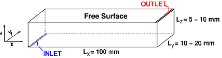
To model the fluid flow that develops prior to the onset of precipitation in our earlier experimental studies14,21, we keep the physical quantities in their dimensional form with the exception of the composition parameter (c). In the cobalt–oxalate system precipitation starts only after the spreading gravity current has expanded to a radius of 1.5−2.5 cm whereas the mixing zone between the two solutions is in submillimeter range. Therefore transverse instability arises where the curvature at these radii does not play a significant role, i.e., the number of sedimentation lines does not change in the time span of an experiment. Thus without loss of generality we can replace the cylindrical system with a rectangular slab geometry shown in Fig. 2 with 10 cm length to reflect the size of a common experimental setup. Two different liquid heights (Lz) are selected (0.5 cm and 1 cm), while the width (Ly) is taken as 1 or 2 cm with periodic boundary conditions to model a laterally unbound system and a symmetry plane is set at the left edge. Zero gradient for the composition is applied for the rest of boundaries except for the inlet where c = 1 is set. For fluid velocity a fixed value of (0,0,0) is taken at the right edge and the bottom, while at the thin inlet (uin) and
L = 100 mmx
L = 10 − 20 mmy Free Surface
z y
x
L = 5 − 10 mm z
INLET
OUTLET
FIG. 2. Geometric parameters of the model system.
outlet (uout) the normal velocity is adjusted in the range of 0.005−0.01 mm/s and tangential flow is allowed on the top without surface deformation to match experimental observations.
The surface tension does not change with the composition in the related experiments21,36, therefore Marangoni flow is not considered even in the presence of a free surface. Buoyant pressure is used according to ~n· ∇p=−(~n· ∇ρ)(~g·~r) where~n is the unit vector normal to the boundary.
The three-dimensional slab is discretized with equal spacing of δx = 0.4 mm and δy = 0.2 mm, while in the vertical direction a varying cell height with geometric progression is used, giving δz = 0.0156 mm on the bottom and δz = 0.782 mm on the top. For solving the governing equations we apply a finite volume method using the OpenFOAM package37, where our in-house code is based on the PIMPLE solver that merges the pressure implicit with splitting of operators algorithm (PISO)38 and the semi-implicit method for pressure-linked equations (SIMPLE) algorithm with implicit Euler method using time steps of 10−3 s. In the discretization the gradient and the divergence are approximated by Gauss linear, while the Laplacian with Gauss linear corrected formulas. Preconditioned biconjugate gradient method is then used where the preconditioning matrix is constructed by the diagonal incomplete LU method with a relative tolerance of 10−6 for the field variables.
III. RESULTS AND DISCUSSIONS
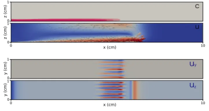
The denser liquid pumped into the thin layer of liquid immediately forms a gravity current and spreads on the bottom. Significant mixing of the solutions only takes place around the large convection roll at the tip where the liquid advancing on the bottom begins to rise abruptly. As shown in Figure 3 for a selected parameter set, the density difference
∆ρ = 0.03−0.15 g/cm3 matching the experimental conditions20,21 produces a very thin layer of expanding fluid current, which generates a substantially weaker return flow in the
upper zone of the liquid layer.
0 0
0 1 1
x (cm) 10
z (cm)z (cm)
0
00 1
1
y (cm)y (cm)
x (cm) 10
FIG. 3. Advancing gravity current for ∆ρ = 0.149 g/cm3, Ly = 10 mm, uin = 0.005 mm/s at t = 300 s: concentration (c) and magnitude of the flow velocity (|u|) in the central vertical xz- plane, lateral (uy) and vertical (uz) components of the velocity field in the horizontal xy-plane at z= 1 mm.
A characteristic height ¯h can be attributed to the gravity current by considering the volume of liquid pumped in and the area covered by the current at a given time (t) according to
¯h= uinAint
Lydx , (3)
where Ain = Ly ×(0.5 mm) is the cross section of the inlet through which the liquid is pumped in with flow rate uin and dx is the extent of the gravity current along the x-axis.
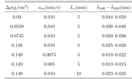
The results summarized in Table I reveal that the characteristic height grows by 10% as the volume of liquid pumped in increases in 400 s. When the density difference between the liquids is increased, the strengthening buoyancy effect above the inlet forces the entering liquid more toward the bottom leading to thinner gravity currents. Decreasing the flow rate of injection at the largest density difference applied causes further thinning of the horizontal currents (see rows 4–6 of Table I), since the smaller vertical momentum of the injected liquid helps the hydrostatic pressure reorient the flow along the x-axis. It is important to point out that the spreading of the injected liquid generates significant fluid flow only at the bottom of the container, therefore doubling the liquid height has only a negligible effect on the characteristic height of the gravity current. Theses findings are in accordance with our observations in earlier experimental studies.21,36The concentration field—and hence the body of the gravity current itself—appears thicker with diffusion as shown in Fig. 3. This is
TABLE I. Characteristic mean height of the gravity current (¯h) for t = 100−400 s for selected parameters (Ly = 10 mm).
∆ρ(g/cm3) uin(mm/s) Lz(mm) ¯h100−¯h400(mm)
0.03 0.010 5 0.044–0.050
0.0559 0.010 5 0.036–0.040
0.0745 0.010 5 0.033–0.036
0.149 0.010 5 0.025–0.028
0.149 0.0075 5 0.019–0.022
0.149 0.005 5 0.013–0.015
0.149 0.010 10 0.023–0.025
more emphasized by inspecting the average concentration alongy-axis, presented in Figure 4 at selected horizontal positions where the concentrations in the figure are given with respect
c/cz=0
0.0 0.5 1.0 1.5 2.0
z (mm)
0 1 2 3 4 5
x=7.2 cm
x = 0.8 cm
FIG. 4. Vertical profiles of mean concentration taken at ∆x= 8 mm from left to right in a gravity current att= 400 s with ∆ρ = 0.149 g/cm3,Ly = 10 mm, Lz = 10 mm, uin= 0.005 mm/s. The concentrations are scaled to the value at the bottom to emphasize the inversion towards the tip.
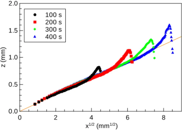
to their values on the bottom (z = 0) to focus on the upward transport. In Figure 4, the concentration profiles vary as we move towards the tip because the injected liquid spreads upwards. The maximum concentration is located on the bottom near the inlet, however, it soon begins to rise. For a quantitative description of this vertical advancement, we can collect the vertical points of inflection in the concentration field above a current, i.e. where
∂2c/∂z2 = 0 and∂c/∂z <0. As the current advances, the upper points of inflection rise with
√xexcept at the thicker head (see Figure 5). This is the result of the coupling between the
z (mm)
0.0 0.5 1.0 1.5 2.0
x1/2 (mm1/2)
0 2 4 6 8
100 s 200 s 300 s 400 s
FIG. 5. Illustration of the vertical diffusional spreading of the upper point of inflection in the concentration field above the gravity current at selected times for Lz = 5 mm. Also shown is the z=√
x line characterizing the pure diffusional transport.
horizontal spreading and the vertical diffusional transport, since the former scales with time and the latter with the square root of time. The characteristic height (¯h) obtained from Eq.
(3) would only match the vertical spreading of the gravity current body in the absence of diffusion which has been reproduced in our model calculations by setting D to zero.
Because of the directionality of the flow, the P´eclet number associated with transport along the x-axis (P ex =Lxux/D >1000) indicates negligible contribution of diffusion only in the horizontal direction. With minimal vertical fluid velocity above the gravity current, the P´eclet number (P ez = Lzuz/D < 5) along the z-axis allows significant diffusional transport between the miscible inner fluid and the freshly pumped in.
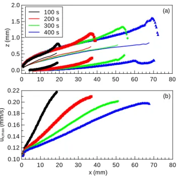
As the injected liquid spreads on the bottom, it drags the initially stationary liquid above it, which also contributes to the thickening of the advancing fluid layer besides diffusion in the vertical direction. Because of the no-slip boundary condition at the bottom, the fluid velocity increases with z before decreasing as we move away from the bottom, leading to an inversion in the concentration field. This generates a second vertical point of inflection, with ∂c/∂z > 0 (see Figure 4). As presented in Figure 6(a), the maximum horizontal fluid velocity is located between the two aforementioned points of inflection. This velocity also
ux,max (mm/s) 0.10 0.12 0.14 0.16 0.18 0.20 0.22
x (mm)
0 10 20 30 40 50 60 70 80
(b)
z (mm)
0.0 0.5 1.0 1.5 2.0
0 10 20 30 40 50 60 70 80
100 s 200 s 300 s 400 s
(a)
FIG. 6. Characteristics of the gravity current at selected times for Lz = 5 mm with ∆ρ = 0.149 g/cm3: (a) points of inflection in the concentration field along the vertical direction indicating the upper and lower extent of mixing, and the location of maximum horizontal flow within (with thin lines); (b) evolution of maximum horizontal flow velocity from injection site with uin = 0.01 mm/s to the tip.
increases from the injection point to the tip of the gravity current as shown in Figure 6(b), a feature also observed in particle-driven gravity currents.30
The maximum horizontal velocity at the head is dominantly the function of the density difference: when it is decreased from 0.149 g/cm3 to 0.030 g/cm3, the terminal horizontal velocity at the tip decreases from 0.20−0.22 mm/s to 0.11−0.12 mm/s. Comparison of these values with those of injection reveals that the advancement of the tip and the large convection roll ahead are fueled by buoyancy in the gravity field. The kinetic energy generated by the injection plays no direct role at these volume flow rates, since it is converted into potential energy as the liquid is pumped upward. Buoyant force will then spread the denser liquid from the vicinity of the inlet in the horizontal direction. At the density differences matching previous experiments,21 the horizontal flow shear above the gravity current remains small compared to the buoyancy term, resulting in Ri > 200, where the Richardson number is
defined asRi=g∆ρLz/(ρ0u2), hence Kelvin–Helmholtz instability does not occur, for which Ri <0.25 is a necessary condition.28
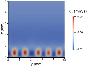
The inversion of concentration field behind the tip furthermore leads to hydrodynamically unstable liquid stratification, since density is a monotonic function of concentration. The formed advancing zone of Rayleigh-Taylor instability generates a row of minor convection rolls in the yz-plane, as illustrated in Figure 3. The cross section in Figure 7, transverse to the main direction of flow, demonstrates that the vortices are centered around the height
0 2 4 6 8 10
0.05
0.00
-0.02 0
2 4 6 8 10
uz (mm/s)
y (mm)
z (mm)
FIG. 7. Vertical component of fluid velocity across the cross section at x = 5 cm characterizing the row of convection rolls behind the tip.
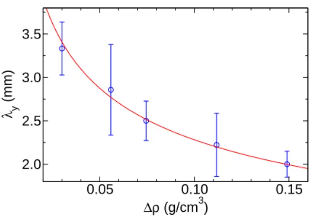
of maximum fluid velocity along the x-axis. In the time frame of the simulation, in accor- dance with experiments, no splitting or merging of the convection rolls is observed. They only exhibit slow transverse motion leading to minor fluctuations around the mean lateral spacing between them due to the finite size of the system along the y-axis. This allows the introduction of a characteristic wavelength associated with the flow pattern; e.g. doubling the width of the system doubles the number of convection rolls but keeps the same spacing between them. The mean wavelength significantly decreases with increasing density differ- ence (see Figure 8), however, it is independent of the liquid height and the velocity of liquid pumped in at higher injection rates.
A dimensional analysis considering the liquid height and the volume flow on injection
0.05 0.10 0.15
∆ρ (g/cm3) 2.0
2.5 3.0 3.5
λ y (mm)
FIG. 8. Variation in the lateral spacing between the convection rolls as a function of density difference. The scaling law based on dimensional analysis is shown with a line.
besides the density difference produces the scaling law λy ∝
νρ0D
∆ρ g 13
. (4)
The scaling law in Figure 8 is in accordance with the results of the simulations. The governing equations in Eqs. (1-2) can be cast in dimensionless form by considering the definition of Schmidt number (Sc = ν/D) and Archimedes number (Ar = gρ0∆ρL3z/ν2). With the introduction of a new pressure relative to the hydrostatic pressure (prgh = p−ρ ~g ·~r), we can take advantage of the formula −∇p+ρ ~g =−∇prgh−~g·~r∇ρwhere~g·~r=−g z. This leads to
∂c
∂τ + U~ · ∇c = 1
Sc∇2c, (5)
∂ ~U
∂τ + U~ · ∇U~ = ∇2U~ − ∇p0 + Ar ζ∇c, (6) where p0 = L3zprgh/(ν2ρ0) is the rescaled pressure without the hydrostatic contribution and ζ = z/Lz. The presence of these two numbers as key parameters is in accordance with the dimensionless form of Eq. (4)
λ0y = λy Lz
∝(Sc Ar)−13 . (7)
This demonstrates that the characteristic size of the transverse array of convection rolls is governed by the competition between the advective transport due to buoyant force and the diffusive transport. The effect of the latter is manifested in the resultant gravity current
height: Faster diffusion leads to thicker spreading and hence an increased spacing between the transverse convection rolls.
IV. CONCLUSIONS
The quantitative characterization has allowed us to distinguish three zones around an advancing gravity current with respect to the local mixing of the liquids prior to the ap- pearance of solid particles. When a precipitate reaction is driven by pumping the solution of one component into the horizontal layer of the other, supersaturation occurs where the two liquids come into contact. The spatial distribution of the precipitate will then depend on the relation between chemical and convective time scales. In case of denser injected fluid, the gravity current spreads on the bottom characterized by a large convection roll at its tip, where the originally stagnant liquid is forced upward. This provides an enhanced local mixing and results in the formation of solid particles when the precipitate formation is instantaneous. With fast sedimentation of particles around the rim, a spreading precipitate disk evolves, like in the case of calcium carbonate.17,20 When the nucleation and growth are slower, the settling is perturbed by the transverse flow generated by the ring of Rayleigh- Taylor instability behind the tip. This results in the angular modulation of the amount of precipitate, which is superimposed on the expanding disk, as seen in the formation of calcium oxalate.14 The formation of solid copper oxalate and cobalt oxalate in a supersat- urated solution is sufficiently slow, so that particles only appear in the zone with unstable stratification.13,21,24 The transverse array of small convection rolls restricts sedimentation to regions where the liquid descends, while regions with rising liquid leads to precipitate-free zones. The final pattern hence consists of evenly spaced lines of precipitate expanding radi- ally without the visible circular rim. The spacing between them depends on the height of the gravity current, which is determined by the density-difference between the liquids and the diffusion of solutes. The third mode of mixing occurs at later stages above the body of the gravity current, where diffusive fluxes lead to the evolution of a supersaturated layer.39 The formed precipitate is angularly homogeneous resulting in the ring structure. The coupling of precipitate reactions and the various modes of transport processes with matching times scales not only determines the macroscopic spatial distribution of the final solid material as described above, but also can lead to an additional control of composition and microscopic
structure in bottom-up syntheses.
ACKNOWLEDGMENTS
The paper is dedicated to Prof. Ken Showalter on his 70th birthday as special thanks to him from ´A.T. and D.H. for his guidance as their PhD supervisor. The work of B´ıborka Bohner and Eszter T´oth-Szeles on preparing the experiments for Figure 1 is gratefully ac- knowledged. This work was financially supported by the National Research, Development and Innovation Office (K119795) and GINOP-2.3.2-15-2016-00013 projects. The authors are also grateful to the Hungarian Supercomputer Center, NIIF, and HPC Szeged for the computational facility.
REFERENCES
1I. R. Epstein and J. A. Pojman, An Introduction to Nonlinear Dynamics: Oscillations, Waves, Patterns, and Chaos (Oxford University Press, Oxford, 1998)
2J. W. Mullin, Crystallization (Butterworth-Heidemann, Oxford, 2001)
3L. M. Barge and et al., “From chemical gardens to chemobrionics,” Chem. Rev. 115, 8652–8703 (2015)
4Q. Wang, M. Bentley, and O. Steinbock, “Self-organization of layered inorganic membranes in microfluidic devices,” J. Phys. Chem. C 121, 14120–14127 (2017)
5F. Glaab, J. Garcia-Ruiz, W. Kunz, and M. Kellermeier, “Diffusion and precipitation processes in iron-based silica gardens,” Phys. Chem. Chem. Phys. 18, 24850–24858 (2016)
6S. Cardoso, J. Cartwright, O. Steinbock, D. Stone, and N. L. Thomas, “Cement nanotubes:
on chemical gardens and cement,” Struct. Chem. 28, 33–37 (2017)
7A. Hussein, J. Maselko, and J. T. Pantaleone, “Growing a chemical garden at the airfluid interface,” Langmuir 32, 706–711 (2016)
8J. H. E. Cartwright, J. M. Garc´ıa-Ruiz, M. L. Novella, and F. Ot´alora, “Formation of chemical garden,” J. Coll. and Interface Sci. 256, 351–359 (2002)
9R. Makki, L. Roszol, J. J. Pagano, and O. Steinbock, “Tubular precipitation structures:
Materials synthesis under nonequilibrium conditions,” Phil. Trans. R. Soc. A 370, 2848–
2865 (2012)
10B. C. Batista, P. Cruz, and O. Steinbock, “From hydrodynamic plumes to chemical gardens: The concentration-dependent onset of tube formation,” Langmuir30, 9123–9129 (2014)
11E. Nakouzi, P. Knoll, and O. Steinbock, “Biomorph growth in single-phase systems:
expanding the structure spectrum and ph range,” Chem. Commun. 52, 2107–2110 (2016)
12L. M. Barge, Y. Abedian, M. Russel, I. Doloboff, J. Cartwright, R. Kidd, and K. I.,
“From chemical gardens to fuel cells: Generation of electrical potential and current across selfassembling iron mineral membranes,” Angew. Chem. Int. Ed. 54, 8184–8187 (2015)
13A. Baker, ´A. T´oth, D. Horv´ath, J. Walkush, A. S. Ali, W. Morgan, ´A. Kukovecz, J. J.
Pantaleone, and J. Maselko, “Precipitation pattern formation in the copper(ii) oxalate system with gravity flow and axial symmetry,” J. Phys. Chem. A 113, 8243–8248 (2009)
14B. Bohner, G. Schuszter, O. Berkesi, D. Horv´ath, and ´A. T´oth, “Self-organization of calcium oxalate by flow-driven precipitation,” Chem. Commun. 50, 4289–4291 (2014)
15G. Schuszter, F. Brau, and A. De Wit, “Calcium carbonate mineralization in a confined geometry,” Environ. Sci. Technol. Lett. 3, 156–159 (2016)
16G. Schuszter and A. De Wit, “Comparison of flow-controlled calcium and barium carbonate precipitation patterns,” J. Chem. Phys. 145, 224201 (2016)
17F. Brau, G. Schuszter, and A. De Wit, “Flow control of a + b c fronts by radial injection,”
Phys. Rev. Lett. 118, 134101 (2017)
18E. T´oth-Szeles, G. Schuszter, ´A. T´oth, and D. Horv´ath, “Diffusive fingering in a precipi- tation reaction driven by autocatalysis,” Chem. Commun. 50, 5580–5582 (2014)
19I. Lagzi, ed.,Precipitation patterns in reaction-diffusion systems(Research Signpost, India, 2010)
20B. Bohner, G. Schuszter, D. Horv´ath, and ´A. T´oth, “Morphology control by flow-driven self-organizing precipitation,” Chem. Phys. Lett. 631–632, 114–117 (2015)
21E. T´oth-Szeles, G. Schuszter, ´A. T´oth, Z. K´onya, and D. Horv´ath, “Flow-driven morphol- ogy control in the cobalt–oxalate system,” CrystEngComm 18, 2057–2064 (2016)
22D. Wang, Q. Wang, and T. Wang, “Morphology-controllable synthesis of cobalt oxalates and their conversion to mesoporous co3o4 nanostructures for application in supercapaci- tors,” Inorg. Chem. 50, 6482–6492 (2011)
23A. T´´ oth, D. Horv´ath, ´A. Kukovecz, M. Maselko, A. Baker, S. Ali, and J. Maselko,
“Pathway control in the self-construction of complex precipitation forms in a cu(ii)–oxalate system,” J. Systems Chem. 3, 4 (2012)
24E. T´oth-Szeles, B. Bohner, ´A. T´oth, and D. Horv´ath, “Spatial separation of copper and cobalt oxalate by flow-driven precipitation,” Cryst. Growth Des. 17, 5000–5005 (2017)
25L. Talon, N. Goyal, and E. Meiburg, “Variable density and viscosity, miscible displace- ments in horizontal hele-shaw cells. part 1. linear stability analysis,” J. Fluid Mech. 721, 268–294 (2013)
26M. John, R. Oliveira, F. Heussler, and E. Meiburg, “Variable density and viscosity, mis- cible displacements in horizontal hele-shaw cells. part 2. nonlinear simulations,” J. Fluid Mech. 721, 295–323 (2013)
27M. Ungarish, An Introduction to Gravity Currents and Intrusions (CRC Press, Boca Ra- ton, 2009)
28P. K. Kundu and I. M. Cohen, Fluid Mechanics, 3rd ed. (Elsevier Academic Press, San Diego, 2004)
29H. E. Huppert, “Gravity currents: a personal perspective,” J. Fluid Mech. 554, 299–322 (2006)
30R. T. Bonnecaze, H. E. Huppert, and J. R. Lister, “Particle-driven gravity currents,” J.
Fluid Mech. 250, 339–369 (1993)
31M. I. Cantero, J. R. Lee, S. Balachandar, and M. H. Garcia, “On the front velocity of gravity currents,” J. Fluid Mech. 586, 1–39 (2007)
32F. Haudin, L. A. Riolfo, B. Knaepen, G. M. Homsy, and A. De Wit, “Experimental study of a buoyancy-driven instability of a miscible horizontal displacement in a hele–shaw cell,”
Phys. Fluids 26, 044102 (2014)
33G. Jones and S. K. Talley, “The viscosity of acqueous solutions as a function of the con- centration,” J. Am. Chem. Soc. 55, 624–642 (1933)
34M. Libert´e, “Model for calculating the viscosity of aqueous solutions,” J. Chem. Eng. Data 52, 321–335 (2007)
35R. Zahor´an, ´A. Kukovecz, ´A. T´oth, D. Horv´ath, and G. Schuszter, “High-speed tracking of fast chemical precipitations,” Phys. Chem. Chem. Phys. 21, 11345–11350 (2019)
36B. Bohner, B. Endr˝odi, D. Horv´ath, and ´A. T´oth, “Flow-driven pattern formation in the calcium–oxalate system,” J. Chem. Phys. 144, 164504 (2016)
37H. G. Weller, G. Tabor, H. Jasak, and C. Fureby, “A tensorial approach to computational continuum mechanics using object orientated techniques,” Computers in Physics 12, 620–
631 (1998)
38R. I. Issa, “Solution of the implicitly discretised fluid flow equations by operator-splitting,”
J. Comp. Phys. 62, 40–65 (1985)
39N. Das, B. M¨uller, ´A. T´oth, D. Horv´ath, and G. Schuszter, “Macroscale precipitation kinetics: Towards complex precipitate structure design,” Phys. Chem. Chem. Phys. 20, 19768–19775 (2018)
![FIG. 1. Images of flow-driven precipitate patterns with flow rate of 20 ml/h for (A) calcium carbonate ([Ca 2+ ] = 4.0 M, [CO 3 2− ] = 0.025 M, t = 3 min, width = 19 cm) and (B) copper oxalate ([Cu 2+ ] = 0.8 M, [(COO) 2 2− ] = 0.05 M, t = 7.5 min, width =](https://thumb-eu.123doks.com/thumbv2/9dokorg/1288350.103112/4.918.275.641.209.388/images-driven-precipitate-patterns-calcium-carbonate-copper-oxalate.webp)