Speeding up non-Markovian First Passage Percolation with a few extra edges
Alexey Medvedev ∗ Gábor Pete †
Abstract
One model of real-life spreading processes is First Passage Percolation (also called SI model) on random graphs. Social interactions often follow bursty patterns, which are usually modelled with i.i.d. heavy-tailed passage times on edges. On the other hand, random graphs are often locally tree-like, and spreading on trees with leaves might be very slow, because of bottleneck edges with huge passage times. Here we consider the SI model with passage times following a power law distribution P(ξ > t)∼ t−α, with infinite mean. For any finite connected graphG with a roots, we find the largest number of verticesκ(G, s)that are infected in finite expected time, and prove that for every k ≤ κ(G, s), the expected time to infect k vertices is at most O(k1/α). Then, we show that adding a single edge fromsto a random vertex in a random tree T typically increasesκ(T, s)from a bounded variable to a fraction of the size ofT, thus severely accelerating the process. We examine this acceleration effect on some natural models of random graphs: critical Galton-Watson trees conditioned to be large, uniform spanning trees of the complete graph, and on the largest cluster of near-critical Erdős-Rényi graphs. In particular, at the upper end of the critical window, the process is already much faster than exactly at criticality.
Keywords: temporal networks; near-critical random graphs; Galton-Watson tree; Erdős-Rényi graph; Pólya urn process; spreading phenomena; SI model; First Passage Percolation; bursty time series; non-Markovian processes. MSC2010 classification: 60K35; 60K37: 05C80;
82C99; 90B18
1 Introduction
1.1 Motivation and background
Spreading is one of the most important dynamic processes on complex networks as it is the basis of a broad range of phenomena from epidemic contagion to diffusion of innovations [Ves12,PSCVMV15].
One of the original, and still primary, reasons for studying networks is to understand the mechanisms by which diseases, information, computer viruses, rumors, innovations spread over them [New03].
The spreading problem initially came from epidemiology, and the terminology still remembers these roots: in the simplest spreading model, the two-statesusceptible-infected (SI) model, any particular person can be either in susceptible (S) or in infected (I) state, with the transition rule S → I, meaning that once an infection is obtained, the person stays infected forever. It is usually assumed that initially there is only one infected person.
∗Namur Institute for Complex Networks (naXys), Université de Namur, Rempart de la Vierge, 8, Namur 5000 Belgium and ICTEAM, Université Catholique de Louvain, Av. Georges Lemaitre 4, 1348 Ottignies-Louvain-la-Neuve, Belgium. Email: an_medvedev ‘at’ yahoo ‘dot’ com
†Alfréd Rényi Institute of Mathematics, Reáltanoda u. 13-15., Budapest 1053 Hungary, and Budapest University of Technology and Economics, Egry J. u. 1, Budapest 1111 Hungary. Email: robagetep ‘at’ gmail ‘dot’ com
arXiv:1708.09652v1 [math.PR] 31 Aug 2017
In the usual mathematical model of SI spreading, a rooted connected simple graphG= (V, E, s) is given, with vertices representing people, and edges representing the connections between them, through which the infection can pass. Initially, only the root s ∈V is infected. The edgese∈ E have i.i.d. random positive weightsξ(e), with common distributionξ, representing the passage time of the infection. Infection is then transmitted along the edges from infected vertices to susceptible ones with passage times according to the edge weights (measured from the moment of infecting the first endpoint of the edge). The process runs until all vertices get infected. Alternatively, and this is how the model was first defined in the mathematical community under the nameFirst Passage Percolation (FPP) [HW65], one may consider ξ(e) as the length of the edge e∈ E, and then we can think of some fluid flowing through this random medium at speed 1, starting from the source s. In the two models, SI and FPP, the moment when a vertex is reached by the infection/fluid will be the same. Then, we can measure spreading via two different, but of course closely related stochastic processes: either by(Tk)|Vk=1| , the sequence of times when exactly k vertices are infected in the process, or by (Nt)t>0, the number of vertices reached by time t. In FPP one is typically more concerned with the process(Nt)t>0 (see, e.g., [Kes87]), while in the current paper we consider the process (Tk)|Vk=1| , therefore we will prefer the SI model notation.
The SI spreading model has attracted much attention in the network science community, giving rise to a solid number of papers (e.g., [IM09, KKP+11, MH13, JPKK14, HK14]). In the mathe- matical literature, there has been an enormous number of papers studying this model on various graphs and using various distributions forξ; see, e.g., [HW65,Kes87,FP93,BvdHH10,BvdHH11, BvdHK14,BvdHH17]; two surveys are [AHD15] on the first 50 years of the model on Euclidean lat- tices and [vdH17, Chapter 8] on other graphs. Although originallyξ was typically assumed to have Exponential or Bernoulli distribution, more recently, motivated by the bursty nature of communi- cations in many real networks, ξ with power law distributions pow(α) have also been considered:
P(ξ > t) = 1∧(t/t0)−α, where t0 >0 and α > 0. In this case the model is non-Markovian, which creates many obstacles in studying it; this will be the situation in the present work, as well.
Most sparse (e.g., bounded average degree) random graph models produce graphs that arelocally tree-like: a large neighbourhood of a random root is a tree with high probability, maybe with some extra edges decorating the tree. Typically, supercritical random graph models have been studied, where the unique giant connected component looks locally like a fast-growing supercritical Galton- Watson tree, maybe with decorations. (In more precise terms, the Benjamini-Schramm limit of the giant clusters is an infinite unimodular random tree with average degree larger than 2, or more generally, an invariantly non-amenable unimodular random graph [BS01,AL07]). This local fast- growing tree structure has been used in several works very successfully to understand the behavior of SI and FPP on the entire graph [BvdHK14,BvdHH17,BvdHK17], even with a general absolutely continuous distribution forξ.
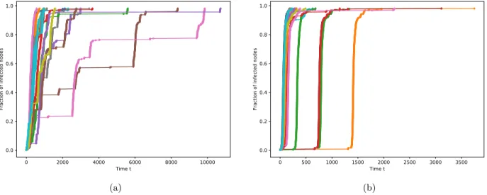
However, it was observed in [IM09] that the SI spreading with heavy-tailedξonfinite trees, when started from a typical site, may be very slow. Real-life examples with such ξ include, for example, information cascades in Twitter [GCSdA+17,BGD+17]. A striking feature of slow spreading when ξ has infinite mean was noticed in [HK14] via computer simulations, which is most apparent when not the curve t 7→ hNti is considered, but the “inverse” curve k 7→ hTki. Namely, running the simulation of the process T = (Tk)nk=1 on a tree for M times, and definining hTki= M1 PM
i=1Tk(i), the spreading curve (hTki, k/n) exhibits “uncontrolled large plateaux”, which do not decrease and do not converge as we increase the number of runs (see the dark blue curves on Figure 1.1 (a)).
Plateaux of similar type were also empirically found in [BGD+17]. On the other hand, adding just one extra edge to the tree (which does not change the local statistics of the graph!) makes the
spreading curve quite smooth; see the lighter green curves on Figure1.1(a), and also Figure1.1(b) that shows SI spreading on the cycle, with power law exponentα∈(1/2,1).
0 500 1000 1500 2000 2500 3000 3500 4000
Time t 0.0
0.2 0.4 0.6 0.8 1.0
Fraction of infected nodes
(a)
0 1000 2000 3000 4000 5000 6000
Time t 0.0
0.2 0.4 0.6 0.8 1.0
Fraction of infected nodes
(b)
Figure 1.1: Spreading curves of the SI model simulation with power law weightsξwithα= 0.8. (a) For the three darkbluecurves, the underlying graph is a tree with472vertices; for the three lightergreencurves, one fixed edge is added between the root and a random vertex; b) the underlying graph is a cycleCnwith472vertices.
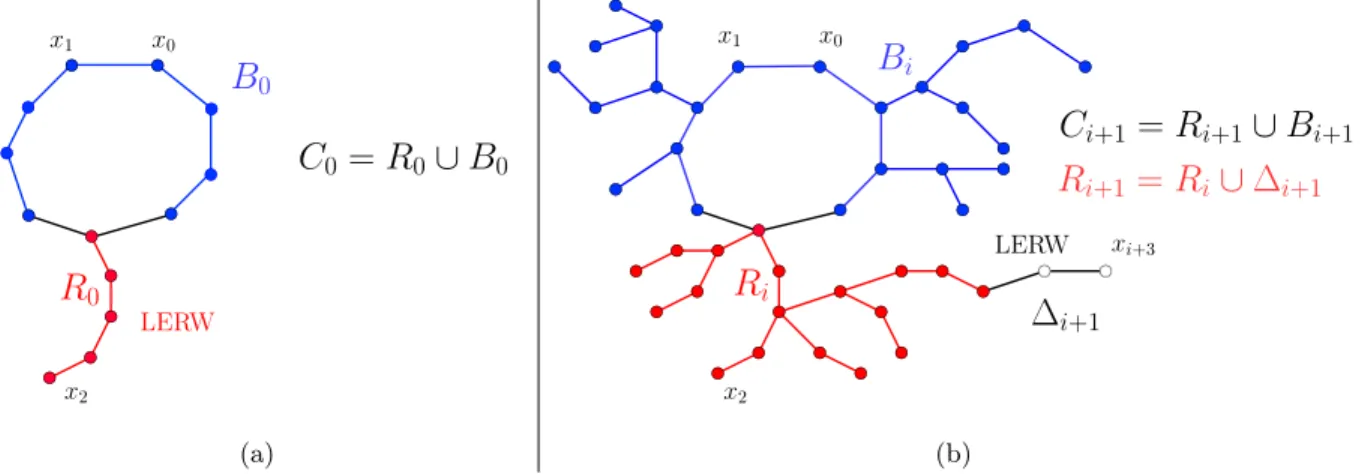
The first motivation for our paper was to understand the striking effect of adding a few edges to large finite trees. After describing this phenomenon in detail for arbitrary deterministic graphs, we address some natural models of random trees, using a variety of techniques. Since supercritical trees are typically not finite (or, if a supercritical GW tree is conditioned to be finite, it becomes subcritical [LP16, Section 5.7]), the most natural and interesting case seems to be adding a random edge to a critical random tree, conditioned to be large in one way or another. Or, in the most natural model that we will consider, the largest cluster in anear-critical Erdős-Rényi graphG n,n1 +n4/3λ
, for λ0is very likely to be a large critical tree, while for λ0is very likely to be a critical tree with several extra edges (see Section 6for references). In particular, the SI process with power law weights forλ 0 is slow and has uncontrolled large plateaux, while most of the graph is infected in a fast and smooth way for λ0(see Figure6.1).
The plateaux are explained by the presence of so-called temporal “bottlenecks”, which are large passage times that occur on some particular edges. Indeed, if there is akfor whichE(Tk)<∞ but E(Tk+1) =∞, then the Law of Large Numbers tells us that
1 M
M
X
i=1
Tk+1(i) −
M
X
i=1
Tk(i)
!
→ ∞a.s., as M → ∞,
and hence the first uncontrolled plateaux in the spreading curve is between hTki and hTk+1i. The next plateau occurs as if we started the process anew after the first bottleneck, without the already infected part of the graph. Hence all the later plateaux can be investigated with the method we describe below, and here we will focus on the time when the first plateau appears.
It is easy to obtain some intuition how the temporal bottlenecks disappear for the SI process on the cycle with α ∈(1/2,1): there are always at leasttwo edges through which the infection might proceed, and the minimum of two independent pow(α) variables already has a finite expectation.
In fact, we will show in Subsection 2.1 that E(Tk) k1/α < ∞ for every 1 6 k 6 n. However, because of the non-Markovian nature of the process (with already old edges getting occupied even later), making such an argument rigorous for a general graph with cycles is not at all trivial.
In any case, we see that for cycles α = 1/2 must be a threshold, and in the current paper we will concentrate on the case of α ∈(1/2,1). Nevertheless, our results can be extended to the case
when the infection hasd >2 ways to proceed andα >1/d; simplistically, the main reason for this bound is that then the minimum of d independent pow(α) variables has a finite expectation. See Subsection1.3 for more details.
1.2 Results and outline
Summarizing the above assumptions, in this paper we consider the SI spreading model with i.i.d.
power law transmission times and we study the role of cycles in speeding up of the process when α∈(1/2,1)and thus eliminating large plateaux on (or ‘smooth’) the average spreading curve up to a certain level. We rigorously identify when the first possible temporal bottleneck appears and its relation to the graph structure. We show that for each finite connected graphGonnvertices there exists a specific thresholdκ(G, s), wheresis an initially infected vertex, such that the average time to infectk6κ(G, s)vertices is finite, and is even bounded by a polynomial function ink, and when k > κ(G, s) the average time is infinite. The result, proved in Section 3, can be stated as follows.
Theorem 1.1. Consider a graph G on n vertices with a root s and the SI spreading process T = (Tj)nj=1 with power law weights with α ∈ (1/2,1). Then there exists the number κ(G, s) such that for eachk, where 16k6κ(G, s), the expected time to infect k vertices is bounded by
E(Tk)6Ck1/α, and fork > κ(G, s), the expectation E(Tk) =∞.
The number κ(G, s) identifies the position of the first temporal bottleneck for the process, and has a simple combinatorial description, which is presented in the following Lemma.
Lemma 1.2. Let G be a finite rooted graph with root sand let T be the SI spreading process onG with weights having absolutely continuous distribution ξ, such that E(ξ) =∞. Then,
κ(G, s) = min
e∈E(G)|C(s, G\e)|,
where |C(s, G\e)| is the size of the connected component of vertexsin the graph Gwithout edge e.
In Section 2, we will describe two examples, the cycle and the star graph, for both of which we have κ=n−1and E(Tκ)n1/α, but for quite different reasons. We have been unable to identify either of these examples as the “hardest graph to infect”, which can be considered as an explanation for the non-triviality of Theorem1.1.
Next, we will study the value of κ(G, s) in some near-critical random graph models, and show that by adding one or a few edges, it increases from a bounded value to a positive proportion of all the vertices. In our first example, we add an extra edge to acritical Galton-Watson treeconditioned to have depth at least N, between the starting vertex s and a uniform random vertex. Here our main tool is comparison with the critical GW tree conditioned to be infinite [Kes86], and our goal is to be as elementary as possible, to develop arguments that may be applicable to other critical random tree models that one may be interested in (see Section4). In our second example, we add one random edge to theuniform spanning treeof the complete graph; this model makes it possible to use elegant methods relying on Loop-Erased Random Walks (via Wilson’s algorithm [Wil96]) and Pólya urns with time-dependent increments [Pem90], very different from the first example (see Section5). Finally, our third example is the “physically” most relevant one: thenear-critical Erdős- Rényi graphG n,1n+n4/3λ
, λ∈R. Here the analysis is based on fine understanding of the metric
structure of the graph [ABBG10b], encoded typically as a Gromov-Hausdorff scaling limit using Aldous’ Continuum Random Tree [Ald91b] as a basic building block (see Section6).
In the first two of these models, in order to raise κ(G, s) significantly, it is important that the extra edge is incident tos, or in other words, thatslies in the cycle that we have created. Instead of adding the extra edge, we could have moved sonto the “spine” of the tree, so that there are two disjoint long paths emanating froms, and this would have a very similar accelerating and smoothing effect. So, in these cases, adding the extra edge could just be considered as a simple way to make the starting vertex special. This also makes sense from a practical point of view: if one’s goal is to speed up the infection process, it is easier to create a new link, or to start the infection at two random places (which is almost the same), than finding a special vertex in the graph to start the process. In the third case, near-critical Erdős-Rényi graphs, the starting vertex will not be special, and therefore κ(G, s) will remain of constant order. However, after infecting a tiny portion of the graph, progressing withka little bit (although typically with a hugeTk), we get to a vertex with a large κ, and from there we infect most of the graph in a fast and smooth way.
We now state our exact results for the three near-critical random graph models. In our first example, we add a single extra edgeebetween the initially infected vertexsand a uniform random vertex in a critical Galton-Watson tree T. This graph will be denoted by T+e, while |T | denotes the number of vertices in T.
Theorem 1.3. Let TN be a critical Galton-Watson tree, conditioned on surviving to at least N generations,ZN >0, and consider the SI spreading process with power law weights withα∈(1/2,1).
Then as N → ∞,
(1) the sequence of r.v. κ(TN, s) is tight;
(2) for any ε >0 there exists δ >0, such that P
κ(T+eN, s)
|T+eN| > δ
>1−ε.
Secondly, a similar result, but with a different approach, is provided for the model of uniform spanning tree of the complete graph.
Theorem 1.4. Let UST(n) be the uniform spanning tree of the complete graph on n vertices, and consider the SI spreading process with power law weights with α ∈(1/2,1), with starting vertex s.
Let e be a uniform random extra edge with one endpoint being s. Then, ∀ε >0 there is δ >0 such that, for alln large enough,
P
κ(UST(n)+e, s)
n > δ
>1−ε.
Thirdly:
Theorem 1.5. Let C=C1n(λ) be the largest cluster of the Erdős-Rényi graph G n,n1 + λ
n4/3
. (1) Let σ be a uniform random vertex in C. Then, as n→ ∞, the sequence of variables κ(C, σ) is
tight for any fixed λ∈R: for every >0, if K >0 is large enough, then P κ(C, σ)< K
>1−, for all n > n0(λ, ) large enough.
(2) For everyλ∈Rand >0, there exists aδ0()>0that is independent of λ, and aδ1(λ, )>0 such that
P
δ0|C|< max
s∈V(C)κ(C, s)<(1−δ1)|C|
>1− .
In particular, the spreading curve may have fast smooth parts for a positive proportion of the volume, but the maximum proportion is bounded away from 1.
(3) For every >0, ifλ >0 is large enough, then P
∀x∈V(C) ∃s∈V(C) with kx(s)< |C| andκ(C0x, s)/|C|>1−
>1− ,
where kx(s) is the random number of steps in which the infection from x reachess, and Cx0 is the graph we obtain from C by removing the vertices infected before s.
1.3 Extensions and open questions
According to Lemma1.2, the first bottleneck appears in the place where the graphGhas a bridge. It is a simple corollary that if the graph is 2-edge-connected, then it contains no temporal bottlenecks for the infection, which is specifically true for a cycle.
It is possible to extend the result of Theorem 1.1 to the case of α ∈(1/d,1), when d > 2, by defining for each finite connected graph Gwith a rootsthe number
κd(G, s) = min
e1,...,ed−1∈E(G)|C(s, G\{e1, . . . , ed−1})|.
Then, for everyk≤κd(G, s), the expected time to infect kvertices satisfiesETk ≤Ck1/α. In order to obtain this result, one would first extend Lemma 3.2to
E
min{X, Y1−t, . . . , Yd−1−t}
Y1, . . . , Yd−1 > t
t1−α,
which has the same order of magnitude as before. Then, in Section 3.2, one should use the delayed process with always having d active edges in the front, and the Q process with d−1 always old edges, getting the bound ETk ≤ Ck1/α at the end. However, it is less clear how to extend our speed-up results. In this case, the bottleneck-free subgraphs are d-edge-connected, hence adding an extra edge and creating a cycle may not always have a speed up effect, and more sophisticated constructions would need to be introduced.
We have explained above why it is natural to consider critical random trees. Nevertheless, one could also condition a subcritical GW tree to be large, and then, depending on the offspring distribution, one would get a tree either very similar to a long path (with tiny trees hanging from it), or to a large star-graph (many spikes, all of bounded depth) [Jan12], so in fact our two introductory examples basically cover subcritical trees, already. For supercritical GW trees, our questions are already not interesting: on the one hand, adding a single edge to an infinite tree has certainly an insignificant effect; on the other hand, as discussed above, for supercritical graphs there is a quite universal and fast spreading behaviour [BvdHH17], where a large tail for ξ does not produce new phenomena.
About the models we have considered, one could also ask more detailed questions. Is there a distributional scaling limit for the process on a critical Galton-Watson tree conditioned to have depth at least N? Time should be scaled by N1/α, as for an iid sum of these variables (FPP on a half-line). And what is the scaling limit on the line segment[−N/2, N/2], started from the origin, time scaled by N1/α?
In the proof of Theorem 1.5, part (1), we are basically showing that the largest cluster of G n,n1 + λ
n4/3
, viewed from a random vertex, resembles a critical GW tree conditioned to have large depth, and then we can use part (1) of Theorem 1.3. With more work, one should be able to show that the Benjamini-Schramm limit of the largest clusteris in fact a GW tree with Poisson(1) offspring, conditioned to be infinite. Surprisingly, we have not found a proof of this in the literature.
Beyond the upper end of the critical window, the results of [DKLP11] do imply this claim.
1.4 Notation
Given two random variablesX1andX2, taking values in some spacesX1andX2, the random variable ( ˆX1,Xˆ2) with values inX1× X2 is a coupling of them if Xˆi has the same marginal distribution as Xi for i= 1,2, i.e., if P( ˆXi∈E) =P(Xi∈E) for all measurable subsetsE ofXi.
If X and Y are two discrete random variables on the same space X, with distributions P(X =x) =px, P(Y =y) =qy, x, y∈ X,
then thetotal variation distance between the measures p andq is dT V(p, q) = 1
2 X
x
|px−qx|= infn
P( ˆX6= ˆY) : ( ˆX,Yˆ) is a coupling of X andYo .
The second equality is usually referred to as Strassen’s theorem (see e.g. [Str65] or [vdH16], p.59).
If X and Y are two real-valued random variables, we say that Y stochastically dominates X, denoted asX Y, if for every x∈R, the following inequality holds:
P(X >x)6P(Y >x).
Stochastic dominationX Y impliesE(X)6E(Y). We use the fact [Lin99] thatX stochastically dominates Y if and only if there is a coupling ( ˆX,Yˆ) ofX and Y such thatP( ˆX>Yˆ) = 1.
If f and g are real-valued functions defined on N or R, then f g and f = Θ(g) mean that there exist constants 0 < c < C < ∞ such that cf(x) < g(x) < Cf(x) for all x. We write f ∼ g, as x → x0, to mean that limx→x0f(x)/g(x) = 1, and write f = o(g) to mean that limx→x0f(x)/g(x) = 0.
2 Two basic examples
2.1 Spreading on a cycle
Consider the example of SI spreading with power law weights on the cycleCn withnvertices, with α∈(1/2,1). The process on the cycle can be understood via the process on the integer line Z: the timeTk of the infection of thek’th vertex has the same distribution onZas onCn, for everyk6n. OnZ, we will denote byXi the power law distributed random weight on the edge(i−1, i)if i >0, and on the edge(i, i+ 1)if i <0.
Proposition 2.1. For the SI spreading process (Tk)∞k=1 on Z with power law weights α∈(1/2,1), the expected time to infectk vertices satisfies
E(Tk)k1/α, where the constant factors depend only on α.
Proof. LetSk= Pk
i=1
Xi and Sk∗= −kP
i=−1
Xi. Note that
min{Sbk/2c, Sbk/2c∗ }6Tk+1 6min{Sk, Sk∗}.
Then it is enough to prove that E(min{Sk, Sk∗}) k1/α. It is well-known (see [Dur10, Theorem 3.7.2]) that the sumSk ask→ ∞ is in the domain of attraction of the stable lawY with the same parameter α:
P(Sk/k1/α> t)−−−→
k→∞ P(Y > t).
Denote Sk = Sk/k1/α. The convergence is given via the convergence of characteristic functions, where the limit characteristic function is given by [Dur10]:
φY(t) = lim
k→∞φS
k(t) =Csgn(t)exp(−b|t|α), (2.1) where the constants,C−1 =C1 and b >0, depend onα. Hence, in the bounded interval|t|<1the convergence in (2.1) is uniform int, thus we can write
φS
k(t) =Csgn(t)exp(−b|t|α)(1 +o(1)),
whereo(1)→0ask→ ∞uniformly in|t|<1. Using the relation between the tail distribution and the characteristic function, given by the following inequality [Dur10, Eq. (3.3.1)]:
P(|X|>2/u)6 1 u
Zu
−u
(1−φX(t))dt,
whereXis a random variable with characteristic functionφX(t), we derive that whentis sufficiently large then for allk,
P(Sk> t)6t
2/t
Z
−2/t
1−(1 +o(1))Csgn(t)exp −b|x|α dx < t
2/t
Z
−2/t
C2|x|αdx=C3t−α, (2.2)
whereC3>0is constant that depends on α. Thus we have for sufficiently larget: P(min{Sk, Sk∗}/k1/α> t)6C4t−2α,
whereC4>0is constant that depends onα. SinceSkis positive then we can find a random variable Z with power law tail with exponent 2α such that |min{Sk, Sk∗}/k1/α|< Z a.s. for all k >0, and thus by Dominated Convergence Theorem forα >1/2 we have convergence of expectations
E(min{Sk, Sk∗}/k1/α)−−−→
k→∞ E(min{Y, Y∗}).
whereY, Y∗ are stable with parameterα. The minimum of Y, Y∗ has power law tail with exponent 2α thus has finite expectation and we have:
E(min{Sk, Sk∗}/k1/α)1, for allk >0, which implies the statement of the proposition.
2.2 Spreading on a star
The star graphStn consists of a distinguished root vertex 0and vertices {1,2, . . . , n−1} attached to it. On Stn, we consider the SI spreading process T = (Tk)nk=1 started from the root, with power law distributed random weights withα∈(1/2,1), denoted asX1, X2, . . . , Xn−1.
Proposition 2.2. On the graphStnwithn>2, the expected time to infectkvertices, fork6n−1, is bounded by
E(Tk)6Cαk1/α,
where Cα >0 is a constant that depends only on α. For k =n−1, in order to infect all but one vertices, we have
E(Tn−1)n1/α, with the implicit constant factors depending on α.
Proof. Denote byX(1)n−1 <· · ·< X(n−1)n−1 the order statistics ofX1, . . . , Xn−1. Then we haveTk+1= X(k)n−1, and it is obvious that
X(k)n−1 X(k)k+1,
for k6n−2, hence the second statement of the theorem implies the first one.
It is straightforward to calculate the tail distribution of X(k)k+1: P X(k)k+1> t
= 1−P(X(k)k+1< t)
= 1−(k+ 1)P(X1, . . . , Xk < t, Xk+1 > t)−P(X1, . . . , Xk+1 < t)
= 1−(k+ 1)(1−t−α)kt−α−(1−t−α)k+1.
(2.3)
To get an upper bound on E(X(k)k+1), we integrate (2.3) overt >0, using the bound(1−t−α)k>
1−kt−α for t > k1/α, and the boundP(X(k)k+1 > t)61 for t < k1/α. After cancellations,
E X(k)k+1 6
k1/α
Z
0
1dt+ (k+ 1)k
∞
Z
k1/α
t−2αdt
=k1/α+ (k+ 1)kk1/α−2
2α−1 6Cαk1/α.
In order to get a lower bound, we use the bound (1−t−α)k<1−kt−α+12k2t−2α for t > k1/α, and the bound P(X(k)k+1> t)≥0for t < k1/α:
E X(k)k+1
>
k(k+ 1)−(k+ 1)2 2
Z∞
k1/α
t−2αdt−(k+ 1)k2 2
∞
Z
k1/α
t−3αdt
∼ 1 2
1
2α−1− 1 3α−1
k1/α>cαk1/α, with some cα>0. Thus,
E X(k)k+1
k1/α, which finishes proof of the theorem.
3 General deterministic graphs
3.1 Preliminary lemmas
We present here two lemmas that will be used in tandem in the proof of Lemma 3.5.
Lemma 3.1. Let (bn)∞n=1 be a positive sequence that satisfies the following recursive inequality for someC >0 and 0< α <1:
bn+1 6bn+Cb1−αn . (3.1)
Then
bn6dn1/α, with d= max{b1,(αC)1/α}.
Proof. We prove the statement by induction. By definition, the statement holds forb16d. Suppose the statement holds for somen >1: for anykwith16k6n, we havebk6dk1/α. Now rewrite (3.1) as
bk+1−bk 6Cb1−αk .
Making a telescopic sum, then using the induction hypothesis and bounding the sum with an integral, we obtain
bn+1−b1 6
n
X
k=1
Cb1−αk 6
n
X
k=1
Cd1−αk1/α−1 6
n+1
Z
1
Cd1−αx1/α−1dx
=αCd1−α
(n+ 1)1/α−1 6d
(n+ 1)1/α−1 .
(3.2)
Addingb1 6dto this inequality, we arrive atbn+16d(n+ 1)1/α, as desired.
Lemma 3.2. LetX andY be i.i.d. power law distributed random variables withα∈(1/2,1). Then, for any t >1:
E(min{X, Y −t}|Y > t)t1−α, with the constant factors depending onα.
Proof. The conditional tail distribution of the minimum is the following:
P min{X, Y −t}> s
Y > t
= P(X > s, Y > t+s) P(Y > t) =
s−α
1 +s t
−α
, if s >1;
1 +s t
−α
, if 0< s <1.
Using the substitutionu= s
t we write the expected value as follows:
E(min{X, Y −t}|Y > t) =
∞
Z
0
P min{X, Y −t}> s|Y > t ds
=
1
Z
0
1 +s
t −α
ds+t−α
∞
Z
1
s t
1 +s
t −α
ds
=t
1/t
Z
0
(1 +u)−αdu+t1−α
∞
Z
1/t
(u(1 +u))−αdu.
In the first integral, 161 +u62, hence that integral is1/tand the term is altogether 1. To calculate the second term, we split the interval of integration into two parts again:
t1−α
∞
Z
1/t
(u(1 +u))−αdu=t1−α
1
Z
1/t
(u(1 +u))−αdu+
∞
Z
1
(u(1 +u))−αdu
. (3.3) The first integral on the RHS of (3.3) is less than R1
0 u−αdu = 1−α1 . The second integral can be bounded in the following way:
∞
Z
1
(1 +u)−2αdu6
∞
Z
1
(u(1 +u))−αdu6
∞
Z
1
u−2αdu,
which is clearly 2α−11 . Summing up the three terms we have calculated, we have proved the lemma.
3.2 Model and main result
We consider finite simple connected rooted graphs G = (V, E, s) on n vertices with m edges. We denote by V(G) the vertex set of G and by |G| the total size of it, or |G|= |V|. We call a path between sand tan (s, t)-path. The graph distance d(s, t) between vertices s andt as the length of the shortest (s, t)-path.
Denote the weight, or the infection passage time, attached to the edgee∈EasXe, whereXeis defined on the probability space(R+,F,P). The probability spaceΩ = (Rm+,Fm,Pm) is the space of all possible random assignments of weights to edges of the graph G equipped with the product measure. Denote byP(s, t)the shortest weighted(s, t)-path and by|P(s, t)|the total weight of this path. The SI spreading process on the graph G is a stochastic process T ={Tk :k∈ {1, . . . , n}}, whereTk is defined as the minimum overHk∈ Gk of the maximum over verticest∈V(Hk) of the total weight of the shortest weighted(s, t)-path. In symbols,
Tk = min
Hk⊂Gk max
t∈V(Hk)|P(s, t)|,
whereGk is the set of subtrees ofGonkvertices with the same root s. We call an edge asoccupied at timet, if both end vertices are in the infected state I, unoccupied, if both are in the susceptible state S, andactive, if one is in stateI and the other is in state S.
The process T is defined on the space Ω, equipped with natural filtration F = {Fk : k ∈ {1, . . . , n}}. Denote the sample sequence T(ω) = {Tk(ω) : k ∈ {1, . . . , n}}, where ω ∈ Ω. Each sample sequenceT(ω), ω∈Ω, defines an orderT(ω)= (e1, e2, . . . , em) on the edge set, in which the edges are occupied by the process. GivenTk(ω)we define for eachktheinfection trail tree G(Tk(ω)) as the subtree from Gk that consists of those edges that successfully passed the infection, i.e., the occupied edges on the shortest paths between the rootsand allk−1other infected vertices. It may happen that at some time Tk(ω) two or more edges, incident to a newly infected vertex, become occupied at the same time. In this case we assume that first the edge on the shortest (weighted) path to the root is occupied, and the rest are occupied with respect to some fixed generic order on the edge set to eliminate ambiguity. Also it may happen that some vertex has two or more shortest paths with equal total weight, but since the system is finite, this event happens with zero probability.
In the current framework, for each ω∈Ωthe spreading curve is the set of pairs {(E(Tk), k/n) : 1 6 k 6 n}. Our goal is to mathematically define the position of the first temporal bottleneck, responsible for the plateau on the spreading curve. Further we restrict ourselves to consideration of power law distributed weights with α ∈ (1/2,1), however some lemmas consider broad class of weights.
First temporal bottleneck. Remember we call an edge active at time t if one of its incident vertices is in state S and the other is in state I. In other words, an active edge is an edge that currently transmits an infection. Let ω ∈ Ω and the front of the epidemic F(Tk(ω))be the set of edges, that are active at time Tk(ω), where k ∈ {1, . . . , n}, in the sample sequence T(ω). Define κ(G, s) to be the maximal number of verticesk such that for each sample sequence T(ω) and for each j < k, the front F(Tj(ω)) has at least two active edges. In other words, it is the minimal k such that there existsω∈ΩwithF(Tk(ω))having one or zero active edges. We say the active edge e is old and has age τ > 0 at time t, if the edge has become active at time t−τ. If τ = 0, then an edge is called new. We now prove that if there is a sample sequenceT(ω) and a number i, for which the front of the epidemicsF(Ti(ω))has one active edge, then there is a large plateau at this point on the spreading curve.
Lemma 3.3. Let G be a finite rooted graph and let T be the SI spreading process with absolutely continuous passage times ξ, such that E(ξ) =∞. Let there exists an ω0 ∈ Ω and a number i∈N, such that the frontF(Ti(ω0))has one active edge. Then for eachj, wherei+1 6j6n, the expected infection time is
E(Tj) =∞.
Proof. The sample sequenceT(ω0)defines the order of occupation of the edge setT(ω)= (e1, e2, . . . , em). Since all edge weights have absolutely continuous distribution and the number of edges is finite, there exists a subsetA(ω0) of sample sequences of positive measure with the same order of occupation of edges as in T(ω). More precisely, there exists a small ε >0 such that the set:
A(ω0) ={ω:|Xej(ω)−Xej(ω0)|< ε},
which has positive measure for any ε > 0. For this, one can take ε to be smaller than half of the minimum of all the absolute differences between the edge weights of different edges (which is almost surely positive).
Then, since the frontF(Ti(ω0))has one active edge, then for eachω∈ A(ω0), the frontF(Ti(ω)) also has one active edge, saye. Therefore, we have
E(Ti+1−Ti| A(ω0)) =E(Xe) =∞, and by the law of total expectation
E(Ti+1) =E(Ti+1−Ti) +E(Ti)>E(Ti+1−Ti | A(ω0))P(A(ω0)) =∞.
Since Ti Ti+1 for all i, then we haveE(Tj) =∞, for all j > i+ 1, which finishes the proof of the lemma.
By Lemma3.3,κ(G, s)captures the exact number of nodes that are infected before the possible emergence of the first plateau. It has a simple combinatorial description, as we stated in Lemma1.2.
Proof of Lemma 1.2. Suppose that there exists ω ∈ Ω and the number k, where 0 < k < n, such that F(Tk(ω)) has one active edge e ∈ E. Then at time Tk(ω) we can divide vertices of G into two classes: infected (in state I) and susceptible (in state S). In the induced subgraph on infected vertices all edges are occupied, and in the subgraph on susceptible vertices all edges are unoccupied, and since the only edge is active, then it is the only one edge between these two subgraphs. Hence, the active edgee is a cut edge, and the size of the infected subgraph equals tokinf =|C(s, G\e)|.
Sinceκ(G, s)is defined as the minimum overω∈Ω, hence can be a bottleneck edge in the process, thus
κ(G, s) = min
e∈E(G)|C(s, G\e)|. This finishes the proof of the Lemma.
Delayed processT. Fix an arbitrary order on the edge set= (e1, e2, . . . , em). Define the process T ={Tk :k∈ {1, . . . , n}}, coupled with the original process T as follows. Start with the infected root s. Then choose the two active edges incident to s with smallest indices in the order and spread the infection through them. At the time when one of these edges becomes occupied, choose the next active edge fromE with the smallest index inand repeat the procedure. If the two active edges share one susceptible vertex, then, when one edge gets occupied, choose two new active edges, given by the smallest indices in . The process runs until there are no more new active edges to take, and the remaining times are assumed to be infinite.
Obviously, for each k < κ(G, s)and each ω∈Ωthe front F(Tk(ω))has two active edges, since the delayed process can be turned into a particular realization of an original process with order of edge occupation .
The process T stochastically dominates the processT, which is proved in the following lemma.
Lemma 3.4. Let G = (V, E, s) be a finite connected rooted graph and let T be the SI spreading process on G with absolutely continuous passage times ξ. Then the delayed process T stochastically dominates the process T.
Proof. Consider anω ∈ Ω. Then for any k, where 1 6k6n, the sample sequence of the delayed process Tk(ω) induces the infection trail treeG(Tk(ω))and we have
Tk(ω) = max
t∈V(G(Tk(ω)))|P(s, t)|.
On the other hand, the original process is given by the minimum over all possible subtrees on k vertices:
Tk(ω) = min
Hk∈Gk max
t∈V(Hk)|P(s, t)|. Therefore, we have Tk(ω)6Tk(ω) for allk, and, hence, T T.
Despite the fact that the delayed process runs slower than the original, the next we define the process Q, which is even slower, but is necessary to achieve our final statement.
Process Q. Define the Q= {Qk :k ∈ {1, . . . , n}} to be the stochastic process, in which at each timeQk there are two active edges with weights X and Y in the front: one of them is always old, with the age of the process, and an other is new. In symbols, let
Q1 = 0,
Q2 = min{X, Y},
Qk+1 =Qk+ min{X, Y −Qk|Qk, Y > Qk},
(3.4)
where the unconditional X, Y are i.i.d. edge weights. The process Q qualitatively constitutes the particular scenario the infection can spread on Z, having an ever old edge Y and spreading only along new edgesX in one direction. The following lemma provides a bound on the expected time to infect kvertices in the process Q.
Lemma 3.5. Consider the process Qk defined above in (3.4) with X, Y ∼ pow(α). Then, for α∈(1/2,1)and for each k, where k>1, we have
E(Qk)6dk1/α. where d >0 is a constant that depends on α.
Proof. Using the law of total expectation, Lemma 3.2and Jensen’s inequality we have that E(Qk+1) =E(Qk+ min{X, Y −Qk}) =E(Qk) +E E(min{X, Y −Qk}|Qk)
6E(Qk) +CE(Q1−αk ) 6E(Qk) +CE(Qk)1−α,
whereC >0is a large enough constant. Then immediately we haveE(Qk)6bk, wherebkis defined with a recursion
bk+1 =bk+Cb1−αk , b1=E(Q2) = 2α
2α−1 6(αC)1/α:=d.
By Lemma 3.1, this sequence is bounded and we have for any k>1: E(Qk)6dk1/α.
This finishes the proof of the lemma.
Define the random variable Xs with the following probability measure:
P(Xs> t) :=P(X−s > t|X > s),
where s > 0. We call the random variable X to have shifted power law distribution shiftpow(α) with α > 0, if P(X > t) = (t+ 1)−α, for all t > 0. Notionally, it represents a power law random variable with a shift of a size of the minimum cutoff. Note that for anys >0, if the random variable X∼shiftpow(α) withα >0, thenXs= (sd + 1)X and therefore, for anys1 < s2:
Xs1 Xs2. (3.5)
In other words, if we consider the SI spreading with shifted power law passage times, then the older edges dominate the newer ones. We can now prove the main theorem of this section:
Proof of Theorem 1.1. Let a random variable X ∼ pow(α), then (X−1) ∼ shiftpow(α). Define T(X−1) to be the SI spreading process coupled toT, with shifted power law passage times with the same parameter α as in T. The shift in times is deterministic, hence by time Tk, the process with shifted times is faster than the original process by the cumulative shift of not more thank−1:
Tk−Tk(X−1)6k−1,
and equality holds only if the infection trail tree is a path of length k−1. The cumulative shift depends on the shape of the infection trail tree given by the process at time Tk and can therefore be non-deterministic.
Since for X, Y ∼ shiftpow(α), then by Lemma 3.4 the delayed process T(X−1) with the same weights dominates the processT(X−1), and we have for anyk6κ(G, s):
TkT(X−1)k + (k−1).
Now consider the process Qwith shifted power law weights denoted as Q(X−1). Since in this case the old edges dominate newer ones, the1 process Q(X−1) dominates the process T(X−1), hence we have
TkQ(X−1)k + (k−1). (3.6)
Since the shift is negative, then we have Q(X−1) Q. Hence, we have for each k, where 1 6k6 κ(G, s),
Tk Qk+ (k−1).
By Lemma 3.5we have
E(Tk)6dk1/α+ (k−1)6(d+ 1)k1/α, whered >0 depends onα, which finishes the proof of the theorem.
From the statement of Lemma 1.2 we have the following simple corollary.
Corollary 3.6. Let G be a finite 2-edge-connected rooted graph with root s and let T be the SI spreading process on Gwith power law weights, where 1/2< α <1. Then for each k6n,
E(Tk)6Ck1/α.
Thus, we established the existence of specific number of nodesκ(G, s) for each finite connected rooted graphG, up to which a spreading curve of the SI process with power law passage times with α∈(1/2,1)has no large plateaux. In case of trees, there is an analytic expression forκ. Consider a rooted treeT with rootson nvertices. Let the degree of the root be equal tods. Denote subtrees hanging from the root as T1, . . . ,Tds (see Figure3.1, a)). Then, by Lemma 1.2,
κ(T, s) =|T | −max{|Ti|: 16i6ds}. (3.7) Now add an extra edge ebetween sand a randomly chosen vertex in the tree. Then, we obtain a graph, denoted asT+e, which consists of a cycleCkof lengthkwithN rooted treesT1,T2, . . . ,TN, whereN >ds a.s., attached to it by edgese1, e2, . . . , eN (see Figure 3.1, b)). Then, by Lemma1.2, we have
κ(T+e, s) =|T+e| −max{|Ti|: 16i6N}. (3.8) In the following sections we consider models of random trees, and we use the above formulas to compare how the addition of an extra edge changes κ.
bc
bc bc bc bc
T1
Ti
Tds
T2
s
(a)
s
bc bc bc
bc
T1
Ti
T4 T3
T2 TN
TN−1
bcbc bcbcbc
bc
bcbc e1
e2
e3
e4
e5
ei
eN−1 eN
bc bc bc
bc
Ck
(b)
Figure 3.1: Schematic structure: a) the treeT with the rootshaving degreeds; b) the graph T+e of a treeT with an extra edgee: a cycleCk with hanging trees T1,T2, . . . ,TN. The sizes of triangles represent the relative size of hanging trees.
4 Critical Galton-Watson trees
4.1 Preliminaries
A Galton-Watson (GW) tree T is defined as a geneological tree of a Galton-Watson process hZn: n > 0i of evolution of a particle system and we assume that Z0 = 1 (see e.g. [Jan12] for the introduction). The process is characterized by the offspring distribution ξ, which is assumed in context of the paper to be non-degenerate, integer and have finite variance Var(ξ) < ∞. The process (and the tree) is calledcritical, if E(ξ) = 1.
The GW trees can be viewed as rooted labeled trees. The root of the tree T corresponds to the particle in the generation Z0, and it is denoted by <0>. A generic particle in the generation Zk is indexed as <0, l1, . . . , lk >, where lr >1, 16r 6k. The particles<0, l1, . . . , lk−1, j >, where j = 1,2, . . ., denote the children of the particle <0, l1, . . . , lk−1 >in generation k−1. Of course, not for allj does<0, l1, . . . , lk−1, j >correspond to an actual vertex ofT. LetN(0, l1, . . . , lk−1)be the number of children of<0, l1, . . . , lk−1 > in the process. Then <0, l1, . . . , lk−1, j >is a vertex of T for 16j6N(0, l1, . . . , lk−1).
Denote the set of all GW trees as hGWi and a randomly chosen GW tree asT. The size of T is defined as the number of vertices it contains and is denoted as|T |. It is well known that a CGW tree is almost surely finite (e.g. Theorem 3.1, p. 84, [vdH16]) and the following theorem provides a bound on the size of a CGW tree [Kol86].
Lemma 4.1. LetT be a CGW tree with integer offspring distributionξ, such thatVar(ξ) :=σ2<∞. Then for n→ ∞,
P(|T |=n) = 1
√2πσn−3/2(1 +o(1)).
Theheight H(T) of a GW treeT is the length of a longest path from the root or the maximum N, such that ZN >0. The following limit theorem about the height of the treeT holds [KNS66].
Lemma 4.2. Let T be a CGW tree with offspring distribution ξ, such that Var(ξ) := σ2 < ∞. Then we have,
N→∞lim NP(H(T)> N) = lim
N→∞NP(ZN >0) = 2 σ2.
The following theorem provides an upper bound on the probability of having a tree of height at leastN conditioned on the exact size of this tree [ABDJ13], [Kol86].
Lemma 4.3. Let T be a CGW tree with offspring distribution ξ, such that Var(ξ) := σ2 < ∞. Then there exist positive constantsC and c, such that
P(H(T)>x
|T |=n)6Ce−cx2/n.
We consider the set of CGW trees conditioned on ZN >0, whereN >0, as the subset of trees hGWi with height at least N. Denote this set of conditioned CGW trees as hGW
ZN > 0i. The expected limit size of thek’th generation in such trees is given in the following Theorem [MM78].
Lemma 4.4. Let T be a CGW tree with offspring distribution ξ, such that Var(ξ) := σ2 < ∞. Then we have:
N→∞lim E(Zk|ZN >0) = 1 +kσ2.
Kesten in [Kes86] proved that CGW trees, conditioned on ZN > 0, converge in distribution to an infinite CGW tree T∞, which is the geneological tree of the critical Galton-Watson process conditioned on non-extinction. The infinite tree has the following construction. The tree T∞ has two types of vertices: normal andspecial, with root being special. Normal vertices have offsprings according to independent copies ofξ, while special nodes have a number of offsprings according to the size-biased distributionξˆ, where
P( ˆξ=k) :=kpk,
andk= 0,1,2, . . .. Every offspring of a normal vertex is normal. When a special vertex produces a number of offsprings, one of its children is selected uniformly at random and becomes special, while all other children are normal.
An alternative construction of the tree T∞ is to start by taking an infinite path γ of special vertices from the root, which is called a spine, and then attachν = ˆξ−1 independent CGW trees at each node of the spine. Since each CGW tree is a.s. finite, it follows that T∞ a.s. has exactly one infinite path from the root, viz. the spine.
4.2 Speed of convergence to the infinite tree
We write as (T[k] =T) and (T∞[k] = T) the event that the firstk generations of the tree T and T∞ respectively match the first k generations of a given tree T. Denote by #Tk the size of k’th generation in the treeT. The following lemma holds for the trees T and T∞ [Kes86].
Lemma 4.5. LetT be a CGW tree with offspring distributionξ. Then, for any rooted vertex-labeled treeT of at leastk generations:
Nlim→∞P(T[k] =T|ZN >0) = #Tk·P(T[k] =T).
Then
P(T∞[k] =T) = #Tk·P(T[k] =T).
It is natural that asN → ∞the conditioned treeTN := (T |ZN >0)andT∞w.h.p. start looking similar. The question now is how large (as a function of N) that similar part is. The following useful proposition answers this question. Versions of this proposition, with the tree conditioned to have exactly N vertices, have appeared in [Ker98, Theorem 5] and [Stu15, Theorem 6.5], but we have not found our exact statement in the literature, hence include a proof.
Proposition 4.6. LetTN be a CGW tree conditioned onZN >0andT∞be an infinite CGW tree.
Then, as N → ∞, for any ε >0 there exist δ >0 and a coupling betweenTN and T∞, such that P(TN[δN]6=T∞[δN])< ε.
Proof. In order to prove the statement of the lemma we show that the conditioned measure and the infinite measure are close in total variation distance. First we establish bounds on the conditioned measure. Consider a rooted treeT with heightk, wherek6δN andδ >0is small. Then by Bayes’
formula,
P(T[k] =T|ZN >0) = P(ZN >0|T[k] =T)
P(ZN >0) P(T[k] =T)
= P(ZN−k(1) >0∪ · · · ∪ZN−k(#Tk)>0)
P(ZN >0) P(T[k] =T),
(4.1)
whereZN(i)−k denotes the (N −k)’th generation in the copy of the CGW processZ(i), started from a vertex at level k. By Lemma4.2, for a large enoughN there existsε0>0such that,
2
σ2N(1−ε0)<P(ZN >0)< 2
σ2N(1 +ε0). (4.2)
Also, when N−kis large enough, there existsε1 >0, such that 2
σ2(N−k)(1−ε1)<P(ZN−k(i) >0)< 2
σ2(N −k)(1 +ε1), (4.3) where16i6#Tk. In order to simplify the further calculations we take commonε2:= max(ε0, ε1) instead of ε0 and ε1 in (4.2) and (4.3), and the conditioned measure is denoted as PN(·) :=
P(· |ZN >0).
Upper bound. We use the union bound on the right-hand side of (4.1) and together with (4.2) and (4.3), we obtain
PN(T[k] =T)6 #TkP(ZN−k >0)
P(ZN >0) P(T[k] =T)
< N
(N −k)#TkP(T[k] =T)1 +ε2
1−ε2
.
(4.4)
Therefore, we can write that for small enoughk there existsε3 >0, such that PN(T[k] =T)< N
(N −k)#TkP(T[k] =T)(1 +ε3). (4.5) Lower bound. We rewrite (4.1) using (4.5) as follows:
PN(T[k] =T) = 1 P(ZN >0)
1−P(ZN(1)−k= 0∩ · · · ∩ZN−k(#Tk)= 0)
P(T[k] =T)
= 1
P(ZN >0)
1−(1−P(ZN−k>0))#Tk
P(T[k] =T)
> 1
P(ZN >0) 1−
1− 2(1−ε1) σ2(N −k)
#Tk!
P(T[k] =T).
(4.6)
Since for anyx, wherex >0, we have1−x <exp(−x)<1−x+x2/2, then for any n>1 1−(1−x)n>1−exp(−nx)> nx−(nx)2
2 . (4.7)
We rewrite (4.6) using (4.7) for x=P(ZN−k>0)and n= #Tk as follows:
PN(T[k] =T)> P(T[k] =T) P(ZN >0)
#TkP(ZN−k>0)−1
2(#TkP(ZN−k >0))2
. (4.8)
Now use (4.3) and we obtain:
PN(T[k] =T)> P(T[k] =T) P(ZN >0)
2#Tk(1−ε2) σ2(N −k) − 1
2
2#Tk(1 +ε2) σ2(N −k)
2!
>P(T[k] =T)#Tk N
N−k 1−ε2
1 +ε2 −#Tk C1N (N −k)2
,
(4.9)
whereC1 = (1+ε2σ22) <1/σ2. Therefore, we can write that for small enough kthere existsε4>0 and a boundedC2>0, that depends on σ and ε2, such that
PN(T[k] =T)>P(T[k] =T)#Tk N
N−k−#Tk C2N (N−k)2
(1−ε4). (4.10) Combining the (4.5) and (4.10), and choosing ε5 := max{ε3, ε4}, we obtain the following bounds on the probability PN(T[k] =T):
N
N−k−#Tk C2N (N −k)2
(1−ε5)6 PN(T[k] =T)
#TkP(T[k] =T) 6 N
(N−k)(1 +ε5). (4.11) Total variation distance. Now we bound the total variation distance between conditioned and infinite measures. From the upper bound in (4.11) we obtain that when k is small enough, the following inequality holds:
PN(T[k] =T)−P(T∞[k] =T)6 N
N −k(1 +ε5)−1
#TkP(T[k] =T)
=
N N −k −1
+ N
N −kε5
#TkP(T[k] =T), and, on the other hand, from the lower bound in (4.11) we obtain
P(T∞[k] =T)−PN(T[k] =T)6
1− N
N−k(1−ε5) + #Tk CεN
(N −k)2(1−ε5)
·
·#TkP(T[k] =T)
=
1− N N−k
+ N
N −kε5+ #Tk CεN
(N−k)2(1−ε5)
·
·#TkP(T[k] =T).
Comparing both bounds we see that all summands are positive, except of
1−NN−k
, thus we can inverse the sign it and derive the bound for an absolute value. Summing those bounds over all possible trees of heightk, we obtain
X
T
PN(T[k] =T)−P(T∞[k] =T) 6X
T
N N −k −1
+ε5
N
N−k+ #Tk CεN
(N−k)2(1−ε5)
·
·#TkP(T[k] =T).
(4.12)