8. 7. Precipitation and cloudiness tendencies in the upper Danube catchment and in Europe 70 8.1. Fig. 7.1: Possible meanings starting from world scenario according to MS Word (1997) list of synonyms. Green set words are primary synonyms of ‖scenario‖, violet words are selected synonyms related to the primary ones. 7.1 Methods of investigation ... 71

8.1.1. 7.1.1 Fourier analysis ... 71

8.1.2. 7.1.2 Method of instrumental variables ... 72

8.2. 7.3 Annual cycle of precipitation ... 74

8.3. 7.5 Effect of warming on cloudiness and sea-level pressure ... 77

8.4. 7.5 Broader analysis of trends in cloudiness ... 79

8.4.1. 7.5.1 Data for analysis ... 79

8.4.2. 7.5.2 Statistical methods ... 80

8.4.3. 7.5.3 Spatial distribution of the trends ... 80

9. 8. Analysis of precipitation and runoff in the Eastern Carpathians ... 84

9.1. 8.1. The runoff data ... 84

9.2. 8.2. Parallel precipitation data ... 85

9.3. 8.3. Basic statistics and extremities ... 86

9.4. 8.4 Regression to the hemispherical temperature ... 87

9.5. 8.5 Independent estimations ... 90

9.6. 8.6 Behaviour of the absolute extremes ... 91

10. 9. Effect of local weather on human mortality ... 93

10.1. 9.1 Mortality data, their trend and annual cycle ... 93

10.2. 9.2 The selected weather parameters ... 95

10.3. 9.3 Methodology of the comparison ... 95

10.4. 9.4 Correlation of death rates with weather variables ... 97

11. 10. Climate scenarios by various methods ... 102

11.1. 10.2 Methods providing extreme index scenarios ... 104

11.1.1. 10.2.1 General Circulation Models ... 104

11.1.2. 10.2.2 Mezoscale models ... 104

11.1.3. 10.2.3 Empirical regression ... 104

11.1.4. 10.3 Comparison of changes in the local averages ... 104

11.2. 10.4 Comparison of selected weather extremes ... 105

11.3. 11.1 Introduction ... 110

11.4. 11.2 Specifics of remote sensing in climate science ... 111

12. 12. Satellite observations for climate science. Part II. ... 123

12.1. 12.1 Testing of climate reproduced by models ... 123

12.2. 12.2 Testing of climate model sensitivity ... 124

12.3. 12.3 Effects of documented land use changes in Hungary ... 126

12.3.1. 12.3.1 Albedo estimation methodology ... 127

12.3.2. 12.3.2 Regional specification ... 130

12.3.3. 12.3.3 Land-use series ... 130

12.3.4. 12.3.4 Area weighting ... 132

12.3.5. 12.3.5 Surface albedo tendencies ... 132

12.4. 12.4 Does climate system respect the GAIA-hypothesis? ... 135

13. References: ... 136

14. Matzarakis, A.; Mayer, H. and Iziomon, M. G., 1999: Applications of a universal thermal index: physiological equivalent temperature. Int. J. Biometeorology 43: 76-84 ... 139

15. Oke, T. R., 1979: Boundary Layer Climates. John Wiley and Sons, 372 pp. ... 140

16. van Engelen, A., A. Klein Tank, G. van de Schrier and L. Klok, 2008: Towards an operational system for assessing observed changes in climate extremes European Climate Assessment & Dataset (ECA&D) Report, KNMI, De Bilt, Netherland, 70 p. ... 142

(3)

17. Animations ... 142 18. Films ... 142

(4)

(5)

ATMOSPHERE AS RISK AND RESOURCE

by Prof. Dr. János MIKA

Eszterházy College, Eger, Hungary

This course is realized as a part of the TÁMOP-4.1.2.A/1-11/1-2011-0038 project.

1. 1. Time and space scales

1.1. Extreme weather

(6)

Specific concern at the middle latitudes are caused by thunderstorms, tornadoes, hail, dust storms and smoke, fog and fire weather. These small-scale severe weather phenomena, that are sparse in space and time, may have important impacts on societies, such as loss of life and property damage. Their temporal scales range from minutes to a few days at any location and typically cover spatial scales from hundreds of meters to hundreds of kilometres. These extremes are accompanied with further hydro-meteorological hazards, like floods, debris and mudslides, storm surges, wind, rain and other severe storms, blizzards, lightning. For example, mudslides disrupt electric, water, sewer and gas lines. They wash out roads and create health problems when sewage or flood water spills down hillsides, often contaminating drinking water. Power lines and fallen tree limbs can be dangerous and can cause electric shock. Alternate heat sources used improperly can lead to death or illness from fire or carbon monoxide poisoning.

Extreme events are often the consequence of a combination of factors that may not individually be extreme in and of themselves. Complex extreme events are often preconditioned by a pre-existing, non-extreme condition, such as the flooding that may result when there is precipitation on frozen ground. In addition, non-climatic factors often play a role in complex extreme events, such as air quality extremes that result from a combination of high temperatures, high emissions of smog precursors, and a stagnant circulation. Very often there is a possibility to predict quite accurately the probability of severe weather events and issue warnings, or even close the endangered region temporarily. But, tourists often do not speak the language of the country in which they are spending vacation. They do not know the local signs of danger and some of them do not respect warnings and prohibitions to enter the endangered areas.

Hence, characteristics of what is called extreme weathermay vary from place to place in an absolute sense. The professional surface-based observations of the Global Observing System provide weather measurements, including air temperature, wind speed, wind direction, precipitation, cloud cover, humidity, sunshine hours and visibility, etc. taken regularly over the Globe. Firstly, we list the extreme weather events following the so called synoptic codes, which indicate the events worth observing, forwarding to the prediction centers and archiving.

Operationally observed phenomena In the observation codes the significant events, i.e. candidates for extreme

events, depending on their frequency and impact, are as follows

(http://www.srh.noaa.gov/jetstream/synoptic/ww_symbols.htm): Haze, mist, fog, dust whirl, sand whirl, dust- storm, sandstorm, freezing rain, ice fog, ice needles, ice sleet. drifting snow, blowing snow, depositing rime ice, rain shower, snow shower, shower of hail, thunderstorm (observed lighting and thunder), squall lines, funnel cloud, tornado.

Majority of these events is rare and of significant impact at most places of the world. This may depend on severity of the event, which is in some cases well classified. Considering the low frequency but negative effects of icing, this event is a meteorological extreme in most regions in the world.

Another group of extremes is the appearance of continuous thermodynamic state indicators above or below a certain frequency and/or impact threshold, e.g. temperature below zero, or rainfall above 20 mm. These extremities are comprehended in the next sub-section.

1.2. 1.2 Present Weather Symbols

(http://www.srh.noaa.gov/jetstream/synoptic/ww_symbols.htm):

In this Section the 100 weather symbols will be presented in Table 1.1.

Table 1.1: The 100 present-weather symbols of meteorology are divided into groups.

Codes 00-09: No precipitation, fog, duststorm, sandstorm, drifting or blowing snow at the station at the time of observation or, except for 09 during the preceding hour.

00 01 02 03 04 05 06 07 08 09

(7)

Cloud development NOT observed

or NOT

observable during past hour (not plotted)

Clouds genera lly dissolv ing or becom ing less develo ped during past hour (not plotted )

State of sky on the whole uncha nged durin g past hour (not plotte d)

Clouds generall y forming or develop ing during past hour (not plotted)

Visibility reduced by smoke

Ha ze

Widespre ad dust in suspensio n in the air, not raised by wind at or near the station at the time of

observatio n

Dust or sand raised by the wind at or near the station at the time of the observati onbut no well- develope d dust whirl(s), and no sandstor m seen:

or, in the case of ships, blowing spray at the station

Well developed dust whirl(s) or sand whirl(s) seen at or near the station during the preceding hour or at the time of observation, but no duststorm or sandstorm

Duststorm or sandstorm within sight at the time of observation, or at the station during the preceding hour

Codes 10-19: No precipitation at the station at the time of observation or, except 17, during the preceeding hour.

10 11 12 13 14 15 16 17 18 19

Mist Patches of shallow fog at station, NOT deeper than 6 feet on land

More or less contin uous shallo w fog at station , NOT deeper than 6 feet on land

Lightin g visible, no thunder heard

Preci pitati on withi n sight, but NOT reachi ng the groun d

Precipitation within sight, reaching ground or the surface of the sea, but distant, i.e.

estimated to be more than 3 miles from the station

Precipitatio n within sight, reaching the ground or the surface of the sea, near to (within 3 miles), but not at the station

Thunder heard, but no

precipitatio n at the station

Squall(s) within sight during past hour

Funnel cloud(s) / Tornado(s) during the preceding hour or at time of observation

Table 1.1 cont.

Codes 20-29 General Group: Precipitation, fog, ice fog, or thunderstorm at the station during the preceeding

(8)

hour but not at the time of observation.

20 21 22 23 24 25 26 27 28 29

Drizzle (not freezing) or snow grains not falling as shower(s) ended in the past hour

Rain (not freezing) not falling as shower(s) ended in the past hour

Snow not falling as shower(s) ended in the past hour

Rain and snow or ice pellets not falling as shower(s) ended in the past hour

Freezing drizzle or freezing rain not falling as shower(s) ended in the past hour

Shower(s) of rain ended in the past hour

Shower(s) of snow, or of rain and snow ended in the past hour

Shower(s) of hail, or of rain and hail ended in the past hour

Fog or ice fog ended in the past hour

Thunderst orm (with or without precipitati on) ended in the past hour

Codes 30-39 General Group: Duststorm, sandstorm, drifting or blowing snow.

30 31 32 33 34 35 36 37 38 39

Slight or moderate duststorm or sandstorm (has decreased during the preceding hour)

Slight or moderate duststorm or sandstorm (no appreciab le change during the preceding hour)

Slight or moderate duststorm or sandstorm (has begun or increased during the preceding hour)

Severe duststorm or sandstorm has decreased during the preceding hour

Severe duststorm or sandstorm has no appreciab le change during the preceding hour

Severe duststorm or sandstorm has begun or increased during the preceding hour

Slight or moderate drifting snow (generally below eye level)

Heavy drifting snow (generally below eye level)

Slight or moderate blowing snow (generally above eye level)

Heavy drifting snow (generally above eye level)

Table 1.1 cont.

Codes 40-49 General Group: Fog at the time of observation.

40 41 42 43 44 45 46 47 48 49

Fog at a distance at the time of observati on, but

Fog in patches

Fog sky visible (has become thinner during

Fog sky obscured (has become thinner during

Fog sky visible (no appreciab le change during the

Fog sky obscured (no appreciab le change during the

Fog sky visible (has begun or has become

Fog sky obscured (has begun or has become

Fog, depositin g rime ice, sky visible

Fog, depositin g rime ice, or ice fog, sky obscured

(9)

not at the station during the preceding hour, the fog or ice fog extending to a level above that of the observer

preceding hour)

thicker during the preceding hour)

Codes 50-59 General Group: Drizzle.

50 51 52 53 54 55 56 57 58 59

Drizzle, not freezing, intermitte nt (slight at time of observati on)

Drizzle, not freezing, continuou s (slight at time of observati on)

Drizzle, not freezing, intermitte nt (moderate at time of observati on)

Drizzle, not freezing, continuou s

(moderate at time of observati on)

Drizzle, not freezing, intermitte nt (heavy at time of observati on)

Drizzle, not freezing, continuou s (heavy at time of observati on)

Drizzle, freezing, slight

Drizzle, freezing, moderate or heavy

Drizzle and rain, slight

Drizzle and rain, moderate or heavy

Table 1.1 cont.

Codes 60-69 General Group: Rain.

60 61 62 63 64 65 66 67 68 69

Rain, not freezing, intermitte nt (slight at time of observati on)

Rain, not freezing, continuou s (slight at time of observati on)

Rain, not freezing, intermitte nt (moderate at time of observati on)

Rain, not freezing, continuou s

Rain, not freezing, intermitte nt (heavy at time of observati on)

Rain, not freezing, continuou s (heavy at time of observati on)

Rain, freezing, slight

Rain, freezing, moderate or heavy

Rain or drizzle and snow, slight

Rain or drizzle and snow, moderate or heavy

Codes 70-79 General Group: Solid precipitation not in showers.

70 71 72 73 74 75 76 77 78 79

(10)

Intermitte nt fall of snowflake s (slight at time of observati on)

Continuo us fall of snowflake s (slight at time of observati on)

Intermitte nt fall of snowflake s

Continuo us fall of snowflake s

Intermitte nt fall of snowflake s (heavy at time of observati on)

Continuo us fall of snowflake s (heavy at time of observati on)

Ice needles (with or without fog)

Snow grains (with or without fog)

Isolated star-like snow crystals (with or without fog)

Ice pellets (sleet)

Table 1.1 cont.

Codes 80-89 General Group: Showery precipitation, or precipitation with current or recent thunderstorm.

80 81 82 83 84 85 86 87 88 89

Rain shower(s) , slight

Rain shower(s) ,

moderate or heavy

Rain shower(s) , violent

Shower(s) of rain and snow mixed, slight

Shower(s) of rain and snow mixed, moderate or heavy

Snow shower(s) , slight

Snow shower(s) ,

moderate or heavy

Shower(s) of snow pellets or small hail, slight with or without rain or rain and snow mixed

Shower(s) of snow pellets or small hail, moderate or heavy with or without rain or rain and snow mixed

Shower(s) of hail, with or without rain or rain and snow mixed, not associated with thunder, slight

Codes 90-99 General Group: Showery precipitation, or precipitation with current or recent thunderstorm.

90 91 92 93 94 95 96 97 98 99

Shower(s) of hail, with or without rain or rain and snow mixed, not

Thunderst orm during the preceding hour but not at time of observati

Thunderst orm, slight or moderate, without hail but with rain and or snow at

Thunderst orm, slight or moderate, with hail at time of observati on

Thunderst orm, heavy, without hail but with rain and or snow at time of

Thunderst orm combined with duststorm or sandstorm at time of observati

Thunderst orm, heavy, with hail at time of observati on

(11)

associated with thunder, moderate or heavy

on with slight rain at time of observati on

on with moderate or heavy rain at time of observati on

on with slight snow, or rain and snow mixed, or hail at time of observati on

on with moderate or heavy snow, or rain and snow mixed, or hail at time of observati on

time of observati on

observati on

on

In Fig. 1.1 One can see the most important symbols around the station, taken from the same Internet source as Tab. 1.1: http://www.srh.noaa.gov/jetstream/synoptic/ww_symbols.htm

Figure 1.1: Symbols drawn around a station on the weather maps.

The weather observations, together with above surface observations and intensive observing systems (e.g radiosouns, satellites, etc. see in the animations) are important themselves, however they provide initial state data for the weather forecasting equations. The latter ones are partial differential equations, representing the physical laws of conservation for mass, thermodynamic energy and momentum (Fig 1.2)

(12)

Figure 1.2: Conservation equations driving the atmospheric motions.

Atmosphere is stratified at their various altitudes according to Fig. 1.3a. This forms natural spheres such as troposphere, stratosphere etc., as indicated in the Figure. Tropopause separating troposphere and stratosphere is located at rather different altitudes depending on the geographical latitude (ie. radiation balance) and the actual season, as indicated in Fig 1.3b.

a.) b.)

Figure 1.3: a.) General stricture of the atmosphere from the surface to the Space. b.) examples of stratification in the troposphere and lover stratosphere depending on the geographical latitude and season. temperature stratification with lower values nearer the surface and higher temperatures above it is called (thermal) inversion.

(13)

1.3. 1.3 Time and space scales

Atmospheric objects exhibit fairly arranged space and time scales. Either drawing the meteorological extremes in the space (x-axis) and time (y-axis) system of coordinates (Fig. 1.4a), or doing the same with the atmospheric objects (Fig. 1.4b), we observe a diagonal distribution of the objects of both drawings. This means, small scale objects are generally short lived, whereas large-scale objects spend more time in the atmosphere.

On the other hand it also means that there are no fast developing extremes which cover large areas and also we do not experience long-term individual extremes or objects which threaten just small areas. Fig 1.4a provides a comprehensive list of meteorological extremes, whereas Fig 1.4b is a brief summary of the atmospheric objects leading to the various meteorological extremes.

a.) b.)

Figure 1.4: Characteristic space (horizontal) and time (vertical) scales of a.) weather and climate extremes and b.) atmospheric objects. Sources: a.) Golnaraghi M., 2005, (2006), b.) Oke, 1979.

Weather extremes are immediately caused by specific weather objects. In developing climate extremes circulation processes also play well recognized role. In the following we briefly survey these objects from the largest scale blocking anticyclones to the smallest scale convective systems. Besides these individual objects, there are even longer-time patterns of the circulation, like the El-Nino - Southern Oscillation or North Atlantic Oscillation, which are not individual circulation objects themselves, but which support specific objects to develop.

For example, unusually warm water surfaces in case of an El-Nino event support developing low-pressure systems above the ocean, and, via complex dynamical processes, higher pressure systems above the continent,.

Though long-term climate extremes can statistically be correlated with these objects, we do not characterize these planetary-scale derived indices below.

Anticyclones generally bear pleasant sunny weather, with no strong air motions, but long residence time above a given land area may lead to drying or even drought of the area. The larger the anticyclones are in their horizontal dimensions, the longer their life-time and slower their transition are. The so called blocking anticyclones of the temperate latitudes may remain for several weeks practically in the same position. Having several such objects in a vegetation season may already cause drought.

Temperate latitude cyclones, as large-sale objects, already bear threats of heavy precipitation and strong gradient winds. Warm fronts of temperate latitude cyclones are responsible for low-intensity, but several days‘

long precipitation. Cold fronts of the cyclones may yield large amount and large intensity precipitation.

Convective activity in and around the cold front, caused by upward motion of relatively warm air masses, may enhance the gradient wind sometimes causing extremely strong wind.

Convection is a key to extreme weather events. Starting from small cumulus clouds, possibly developing into single-cell local thunderstorms, they are still not subjects of extremes events. Multi-cell thunderstorms, causing heavy rain, sometimes hail and stormy wind are already extremity-bearing atmospheric objects. Single-

(14)

cell thunderstorms sometimes develop into super-cells, accompanied with devastating wind and hail, heavy rain and often even with tornado. Not so dangerous, but more complicated are the so called mezoscale convective complexes (MCC), often bearing thunderstorm lines, squall lines, characterized by stormy wind, hail and intensive rain.

The most devastating objects of convective origin are the hurricanes (tropical cyclones, typhoons). Their 3-500 km characteristic diameter develops after a large number of coincidental conditions leading to accumulation of very high amounts of available potential energy turning into kinetic energy. In a tropical cyclone, extremely strong winds, intensive rain and hail, with several meters high waves at the shores cause infinite harm.

1.4. 1.4 Climate extremes

Climate extreme is a longer-term mean or frequency of variables or events, even if the latter are not weather extremes, which are rare at the given site in the given time of the year, and which are of potentially high impact.

The climate extremes may be time averages or frequencies of events above a given threshold of a single meteorological variable. These indices are presented below. Those extremes which occur in the multi- dimensional phase-space, but which are mostly transformed into univariate indices, are illustrated afterwards.

Univariate indices. Typical indices include the number or fraction of cold/warm days/nights etc. above the 10th percentile, generally defined with respect to a preselected reference period. Other definitions e.g., the number of days above specific temperature or precipitation thresholds, or those related to the length or persistence of climate extremes.

Table 1.2: Selected examples from the 40 univariate climate indices used in ECA&D. (see http://

eca.knmi.nl/indicesextremes for details, van Engelen, et al., 2008).

Index Climate Index Description

TG, TN and TX

Mean of daily mean, maximum and minimum temperature (°C)

(For further use in the indices)

ETR Intra-period extreme temperature range (°C)

Difference: max(TX)- -min(TN)

GD4 Growing degree days (°C) Sum of TG > 4°C

GSL Growing season length (days) Count of days between first span of min. 6 days TG > 5°C and first span in second half of the year of 6 days TG < 5°C

CFD Consecutive frost days (days) Maximum number of consecutive days TN < 0° C

HD17 Heating degree days (°C) Sum of 17°C - TG

ID Ice days Number of days TX < 0°C

CSFI Cold spell days (days) Number of days in intervals of at least 6 days with TG <

10percentile calculated for each calendar day (on basis of 1961-90) using running 5 day window

WSDI Warm spell days (days) Number of days in intervals of at least 6 days with TX >

10percentile calculated for each calendar day (on basis of 1961-90) using running 5 day window

TN10p Cold nights(days) Percentage or number of days TN < 10percentile calculated for each calendar day (on basis of 1961-90) using running 5

(15)

day window

TG90p Warm days (days) Percentage or number of days TG > 90percentile calculated for each calendar day (on basis of 1961- 90) using running 5 day window

RR Precipitation sum (mm)

RR1 Wet days (days) Number of days RR ≥ 1 mm

SDII Simple daily intensity index (mm/wet day)

Quotient of amount on days RR ≥ 1mm and number of days RR ≥ 1mm

CDD Consecutive dry days (days) Maximum number of consecutive dry days (RR < 1mm) R20mm Very heavy precipitation days (days) Number of days RR ≥ 20mm

RX1day Highest 1-day precipitation (mm) Maximum RR sum for 1 day interval

R95p Very wet days (days) Number of days RR > 95percentile calculated for wet days (on basis of 1961-90)

R95pTOT Precipitation fraction due to very wet days (%)

Quotient of amount on R95percentile days and total amount

In 1998, a joint WMO-CCl/CLIVAR Working Group formed on climate change detection. One of its task groups aimed to identify the climate extreme indices and completed a climate extreme analysis over the world where appropriate data was available. Extreme climate analyses have been accomplished on global and European scales using these compiled datasets. A selection of these indices is given in Tab. 6.1 already from a more recent source using 40 indices (van Engelen et al., 2008).

Multivariate extremities, transformed into univariate indices. Extremity of weather or climate, as well as the effect of them are often more complex than rarity or severity of one single meteorological variable. The use more variables, however, does not allow to establish a linear sequence of the extremities. Hence, most often the multivariate extremities are arranged into a single index.

For example, the thermal comfort index is calculated by means of the physiologically equivalent temperature, PET, based at the human energy balance (Matzarakis et al., 1999). For calculating this weather extreme four meteorological parameters (air temperature, relative humidity, wind speed and cloudiness) as well as some assumed physiological parameters (age, genus, bodyweight and height, average clothing and working) are used.

Our second example on multivariate indices is related to a climate extreme, drought, which is possibly the most slowly developing one. There are many conceptual definitions of drought in the scientific literature. Recently, Dunkel (2009) collected a few of them focusing on the more practical indices from data accessibility point of view. A very commonly used and accepted index is the Palmer Drought Severity Index (Alley, 1984), which considers monthly precipitation, evapotranspiration, and soil moisture conditions.

See also the ANIM_1_1 with the various observation networks and ANIM_1_2 with a series of radar images from a long series of days with precipitation.

FILM_1_1_cloud_webcam.avi presents cloud movements as seen from the surface by a web-camera and from the space by the Meteosat geostationary satellite. The webcameras are operated by the Hungarian Meteorological Service (OMSz).

(16)

FILM_1_2_bootcloud_Italy.mpeg provides a unique set af moving satellite images effectively illustrating that cumulus cloudiness is primarily generated by convection. These clouds form exclusively over the hot Apennine peninsula over Italy in the given situation, but not over the cool sea surface around it.

2. 2. Limitations of macro-circulation objects

(Can water deficits of Lake Balaton in 2000-2003 be explained by circulation anomalies?)

This Section presents a quantitative analysis answering the question put in the brackets. After general exposition of the problem (Section 2.1), the methodological bases of this effort are given in Section 2.2, whereas the quantitative explanation is described and illustrated in Section 2.2. Finally, lack of success in explaining the missing precipitation and assumed consequences related to macro-circulation based statistical downscaling are discussed (Section 2.3).

2.1. 2.1 General exposition

Extreme weather and climate events received increased attention in the last few years,due to the loss of human life and exponentially increasing costs, associated with them (Changnon et al., 1996). At the temperate latitudes, major extremes are connected with irregular water supply of land surfaces by precipitation. Both, flooding or inundation and drought may cause serious damage in hydrological and agricultural objects and values.

Precipitation is connected mainly with mezo-scale atmospheric phenomena and influenced by physical processes of smaller dimensions, including microphysics of cloud droplets and crystals. Hence, deterministic computation of this atmospheric variable is rather limited compared to requirements of medium-range weather forecasts and climate scenarios.

Statistical approaches to derive precipitation fields from synchronous circulation patterns were first applied in medium-range weather forecasting (Glahn and Lowry, 1972; Klein and Glahn, 1974), and later in regional down-scaling (e.g. Bardossy et al, 1995). Both applications are based on the common sense that pressure or geopotential fields can be better predicted by the models, than the short lived precipitation objects. This approach is also useful if one combines daily circulation types with point-wise conditional distributions of precipitation (Bartholy et al., 1995), where patterns are likely better approached, too.

In Europe the cyclone tracks established by van Bebber are presented in Fig. 2.1. Track I is busy in all seasons.

Tracks II and III are engaged mainly in winter, whereas the track 4 make weather forecastersbexcited mainly in summer and autumn. Track V/a delivers cyclones mainly in winter, whereas the track V/b, crossing northward through the region of the Carpathian Basin is mostly engaged in spring and in October. The frequency list is led by track I, where 31 % of the cyclones move along in winter and 39 % in summer. Further positions are taken by tracj IV (12 and 22 %) and track V (13-18%).

(17)

Figure 2.1: Cyclone tracks in Europe (after Van Bebber)

2.2 Methoology

2.1.1. 2.2.1 Statistical assessment using circulation types

In the followings, a method is introduced to calculate the relative contribution of the circulation anomalies, expressed by frequency distribution among finite number of classes, to the climate anomalies. The aim of this method is to quantify what part of climate anomalies can be directly attributed to the anomalous frequency distribution of macro-synoptic types in the period for which the anomaly is formed. Mathematical formulation of this task is as follows:

Let a mark the deviation of diurnal precipitation from its climatic mean in a preliminarily fixed period consisted of M days (e.g. M=30 for monthly, or 90 for seasonal periods). Let us further have k different circulation types, one of them unequivocally being valid at each day of the investigation period. It is also possible to identify the deviation of the frequency related to the j-th circulation type from its climatic average frequency. If having a longer period of diurnal precipitation and also of circulation type series, it is also possible to compute the sign and the amount the conditional precipitation differs from the overall diurnal average in the given period of the year. This average conditional anomaly of precipitation, , can be computed as follows:

. (1)

If the precipitation anomaly of the given period of M days is largely caused by anomalous occurrence of the circulation types, then the observed anomaly, a, and the above anomaly of circulation origin, a*, are of similar value. Earlier investigations, based on different subjective and objective classifications and various target variables for Hungary, established, however, that this circulation term was able to explain just a minor part of the monthly anomalies (Mika, 1993, Mika et al., 2005). On the other hand, according to both papers, the circulation term and the overall anomaly fluctuate in strong correlation with each other.

In the followings terms, a and a*, are compared by using three different classifications described in the following section. Bimonthly periods (Jan-Feb, Mar-Apr, etc.) are investigated considering four consecutive years, 2000-2003. This separation of the months ensures separate treatment of the primary (May-June) and the secondary (November-December) precipitation maxima of the year. For reference period we used the period 1990-1999.

2.1.2. 2.2.2 The applied classifications

Macro-synoptic classification is a description of spatial distribution of the sea level pressure or mid-tropospheric geopotential height by subjective or objective methods. In the followings, the three applied subjective classifications are briefly described. The three classifications are listed in a decreasing order of their spatial scope.

2.1.3. 2.2.2.1 Hess-Brezowsky classification, amalgamated (9 types)

The Hess-Brezowsky (HB) classification (Hess and Brezowsky, 1969), based on the diurnal sea-level and mid- troposphere pressure fields of Central Europe, scoped from Germany, defines 29 different types and allows one class for the rare undefined patterns. The HB-codes are defined operatively by the German Weather Service in

(18)

Frankfurt am Main. Actually, this coding was used until the end of 2001, but from 2002 the operational coding by the Hungarian Meteorological Service was applied in the calculations.

This number of classes, however, is too large for our purposes and sample sizes. Hence, they are objectively compressed into 9 groups, considering the results of a factor analysis (von Storch and Zwiers, 1999), performed for the annual sea-surface pressure maps averaged for each of the 29 HB types (Mika et al., 1999).

These maps had previously been derived by Bartholy and Kaba (1987), who collected diurnal pressure patterns of a 11 years period, and determined average annual mean sea-surface pressure distribution above the continental Europe (2.5 x 2.5 rectangles), i.e. above the area of the HB classification.

Reduction of the HB types is performed by factor analysis of the 30 average pressure patterns. Number of retained factors is determined by the Guttman criterion (Bartzokas and Metaxas, 1993), to keep the factors with eigenvalues>1. Rotation of the axes (factors) is performed by Orthogonal Varimax Rotation, which keeps the factors uncorrelated. This process achieves discrimination among the loadings, that makes the rotated axes easier to interpret.

Number of eigenvectors to retain was definitely four, but cases (i.e. original HB-types) with opposite signs (cyclone, or anti-cyclone above a large of the map) were kept different in the new cumulated classification.

Some cases not unequivocally separated by the factors also occurred, but (the rotated) Factor 3 contributed to each of them with high positive or negative loading. The original unclassified cases are kept separately, though its frequency is rather low.

This methodology contributed to the reduction of the number of macro-types from 30 to 9. Tab. 2.1 demonstrates the new, condensed macro-types. The correspondence between the original and the condensed types is established objectively, without any further synoptic consideration. To follow this correspondence, one could turn to the original paper by Hess and Brezowsky (1969), or to any paper applying this classification (e.g.

Bartholy et al., 1995).

Tab. 2.1: Amalgamation of the 29 primaryHess-Brezowsky types into 9 different classes, according to factor analysis of the mean sea-level pressure patterns (Mika et al., 1999)

Classes Class 1. Class 2. Class 3. Class 4. Class 5. Class 6. Class 7. Class 8. Class 9.

Factors F1: + F2: + F3: + F4: + F1: - F2: - F2-F3:+ F3: - EXTRA

Original HB-types

Sa Sz, SEa Sez, HFz TM

Wa SWa HM BM

Ws Ww TB TRM TRW

NEa NEz HFa

Na Nz

NWa NWz

HNz HNFz

Wz SWz HB HNa HNFa

Egyéb

2.2.2.2 Péczely classification (13 types)

Considering weather situations in Hungary, Péczely (1957) defined a macro-synoptic classification, based on the position of cyclones and anticyclones on the sea-level pressure maps. Thirteen types are separated and grouped according to direction of the prevailing current (Tab. 2.2). The types consider the position of the major frontal systems relative to Hungary, as well. Transition-probability matrices of the different types are given by Péczely (1983) for 1881-1983. Since his death, Karossy (1987 and updated) continues the tradition, determining the actual codes, with the intention to repeat the original macro-circulation identification.

2.2.2.3 Bodolainé classification (8 types)

The aim of the monograph, written by Bodolainé (1983), is to establish the synoptic conditions of flood waves in the Danube and Tisza basins, describing the background of the genesis of floods in terms of synoptic-

(19)

climatology. Weather types with enhanced precipitation activity are analysed, including their distribution in time and space, the watered area and the amounts.

Tab. 2.2: The 13 individual types of the Péczely (1957) macro-synoptic classification. (These types are used according to their serial numbers, i.e 1 for mCc, 2 for AB, …, 13 for type C. The related drawings of Figs. 2 and 3 are marked according to this rule.)

MERIDIONAL TYPES ZONAL AND CENTRAL TYPES

Types connected with westerly current:

Types connected with northern current: zC - zonal flow, slightly cyclonic influence mCc - H is in the rear of a West-European cyclone Aw - anticyclone extending from the west AB - anticyclone over the British Isles As - anticyclone to the south from Hungary CMc - H is in the rear of a Mediterranean cyclone Types connected with easterly current:

An - anticyclone to the north from Hungary Types connected with southerly current: AF - anticyclone over the Fenno-Scandinavia mCw - H is in the fore of a West-European cyclone Types of pressure centres:

Ae - anticyclone to the east from Hungary A - anticyclone centre over Hungary CMw - H is in the fore of a Mediterranean cyclone C - cyclone centre over Hungary

Tab. 2.3: The seven types of the Bodolaine (1983) classification with considerable precipitation. (Serial numbers assigned to the types are used in Fig. 3.)

. West-type-weather situations (W):

· a deep cyclone is situated over North-Europe at mean see level pressure

· strong westerly stream is characterised over the Carpathian basin at 500 and 700 hPa levels.

· the precipitable water is generally higher, than the average.

· The temperature is higher during winter, and cooler during summer.

2. West type with secondary lateral distribution (Wp):

· a deep cyclone is situated over the North-Sea at mean see level pressure

· strong south-westerly stream is over the Carpathian basin at 500 and 700 hPa levels.

· the precipitable water and the temperature is always higher, than the average all the year.

· This is a warm situation in the Carpathian basin.

3. Zonal-type weather situation (Z):

· a deep cyclone is situated relatively far over the North-Sea at mean see level pressure

(20)

· westerly stream is characterised over the Carpathian basin at 500 hPa level.

· Temperature is higher during winter and spring, causing snowmelt in the Alps in this period.

4. Transporting Mediterranean cyclone-type (M):

· a cyclone is situated near or over the Carpathian basin at mean see level pressure

· strong south-westerly stream is characterised over the Carpathian basin at 500 hPa levels

· the precipitable water is much more higher, than the average.

· Considerable part of the annual precipitation amount is connected with this type in Hungary.

5- Centrum-type weather situation (C):

· a deep cyclone over the Carpathian basin both at the see level and at the higher levels, as well

· the precipitable water is always higher, than the average all the year.

· It is a relatively rare situation, but it causes a lot of precipitation in the Carpathian basin.

6. West cyclone type weather situation (Cw):

· a deep cyclone over West Europe at higher level, and over the Alps at mean sea level pressure.

· the precipitable water and the temperature is always higher, than the average all the year.

· This is a warm situation in the Carpathian basin.

7. Cold air –drop weather situation (H):

· This situation is often during summer.

· The curvature of isobars is cyclonic in the Carpathian basin

· The unstable air and high precipitable water are favourable conditions for convective systems.

Classification of the weather-systems of the flood-waves producing rainfall periods can also be found in the monograph. The weather types are defined by the ridge- and trough-lines of the 500 hPa surface, by those of the 500/1000 hPa thickness, as well, as by the near-surface position of cyclones and anticyclones. These types can also be expressively characterised by the mean fields of the precipitable water. Seven circulation types characterised with significant precipitation in Hungary were defined (Tab. 2.3), plus another type without strong precipitation activity was also introduced: The catalogue of the weather types, regarding the period between 1951 and 1980, enabled also the frequency analysis of the types.

For the period after July 2001, the coding was performed by one of the authors (L.P.), performed using 00 UTC maps of 500 hPa and sea-level pressure, published by the German Weather Service web-site, www.wetterzentrale.de, also considering daily precipitation data.

2.1.4. 2.2.3 Point-wise vs. area-mean precipitation

Precipitation directly reaching the Lake Balaton surface is determined from ca. 10 stations, situated in close vicinity of the Lake. The same value for the whole water catchment is derived from ca. 25 stations. Our estimation of circulation component, described in Section 2.1, needs daily precipitation data, which were obtained only for one station, Siofok. Hence, the aim of the following paragraphs is to demonstrate close correlation and near-unity regression between monthly values of this single station, and those for the large areas, including the whole watershed and the lake, as well.

As indicated in Fig. 2.2, both statistical characteristics are fairly close to the unity. Each coefficient is derived from 10 pairs of data between 1990 and 1999. All correlation coefficients between the point-wise

(21)

observations and the area-mean characteristics are above 0.8. (One should note that correlation between lake- mean and watershed-mean precipitation is not always 1, either.) The coefficients are somewhat higher between point-wise observations and lake-mean estimates, but in 4 months of the year (November, January, February and March) even this relation is the opposite.

Point-wise observations can be used for area mean estimates with regression coefficients that are, again, fairly close to the unity, Moreover, regression coefficients between point-wise observations and one or the other area- mean estimates do not deviate from the unity more than the same regression between the two area-mean estimates, themselves.

Hence, the single-station precipitation observations are considered to explain lack of water supply in the 2000- 2003 period in comparison with the previous ten years, 1990-1999.

Fig. 2.2: Correlation and regression coefficients between precipitation falling to the water cathment and the single station (Siófok), between those captured by the lake and, again, the single station, and also between the catchment and the lake captured values. Each coefficient is derived from 10 pairs of data between 1990 and 1999.

2.3. Estimation of precipitation by macro-circulation

2.1.5. 2.3.1 Conditional mean precipitation

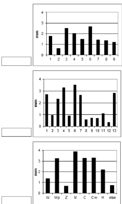
As expected, conditional mean precipitation considerably differs between the classes of a given classification.

This is valid for all the three above classifications (Fig. 2.3).

In case of the condensed HB-classification (Fig. 2.3a) the highest average precipitation sums are accompanied with classes 6, 3 and 4 (see in Tab. 1), representing the frontal section or the axis of a high-level trough with cyclonic curvature above the Carpathian basin. Not surprisingly, the lowest average precipitation occurs in Class 2, which bears mainly anticyclonic situations over Hungary.

For the Péczely-types (Fig. 2.3b) the highest average precipitation sums are accompanied with the cyclonic situations (class 6, 4, 13, 1, 7 and 6, see in Tab. 2.2). The highest amounts are accompanied with warm fronts of the Mediterranean and the Atlantic cyclones. Definitely lower amounts occur in the anticyclonic situations (class 12, 8, 10, 9, 5, 2 and 11, as ordered in the opposite direction).

The Bodolainé-classification (Fig. 2.3c) relates the highest average precipitation sums with transporting Mediterranean cyclones (type M, see in Tab. 2.3) and with three other types characterised by cyclonic curvature or effect of such areas on Hungary. Much lower amounts occur in the zonal types with no meridional disturbances in the region (types Z and W), and in the class ―rest‖, which is not considered to be significant from precipitation point of view.

(22)

To conclude this sub-section, one can establish that higher average precipitation is really connected with cyclonic types, but non-zero conditional averages occur even in the anticyclonic situations, as well.

Fig. 2.3: Mean conditional precipitation, according to the individual macro-synoptic types. 1990-2003, Siófok, Hungary. (Although in process of estimation monthly distinction among the conditional anomalies is performed, the present figures are annual averages.) Siófok, Hungary. (Although in the process of estimation monthly distinction among the conditional anomalies is performed, the presented figures are annual averages.)

2.1.6. 2.3.2 Frequency of the circulation types in 2000-2003 vs. 1990-1999

(23)

The other side of the question, put in the title of the paper, is how much the frequency distribution of the circulation types differed from its average one in the given four years. Parallel columns of Fig. 2.4 indicate these differences in bimonthly resolution. First columns always correspond to the 10-years mean frequency (1990- 1999). The second ones represent the same 2 months of the critical four-year period (2000-2003) with lower than normal precipitation.

Fig. 2.4: Frequency of the given types in the three applied classifications. 10 J-F means January-February 1990-1999, and the next column to the right means the frequency distribution in the given four-year period of drought at Lake Balaton These columns can be analysed to establish quantitative differences between the 4-years and the 10-years periods. Of course, none of the three types exhibit identical distribution of the types in the two periods. For the most critical May-June period, when the lack of precipitation was the most serious, as compared to normal values, surplus of types with low precipitation and lower frequency of highest conditional means were observable. I.e., less frequency of types 3, 4 and 6, but more cases with type 5 can be established in terms of the cumulated HB-types. The same in terms of Péczely classification means below normal frequency of wet types 3, 4 and 6, and above normal occurrence of dry types 5 and 12. Classification by Bodolainé exhibits far more non-significant (―remaining‖) types, but less than normal frequency of types M and Cw.

2.1.7. 2.3.3 Observed vs. circulation-related anomalies of precipitation

(24)

Results of the estimation on effect of circulation, applying formula (3.1), are comprehended by Fig. 2.5.

Comparison of the observed precipitation anomalies with those estimated by the three classifications, unequivocally point at the secondary role of the circulation factor.

Among the six bimonthly periods, January-February and July-August exhibit almost zero anomaly of precipitation during the four years. In these periods the circulation term does not differ much from the observed one. In the other four periods of the year, however, the observed anomalies are poorly approached by the circulation term. In the March-April and November-December periods even signs of the circulation term are positive, contrary to the considerable negative anomalies of the observed precipitation. In September-October the negative observed anomaly is paired by two small negative estimated anomalies (HB and Péczely types) and one larger positive one (Bodolainé types). Hence this estimation is not good either.

Sign of the anomalies is correctly reflected only in the most critical May-June period, with 1 mm/day negative anomaly (i.e. 60 mm/2 months, or 240 mm in the four May-June periods of 200-2003). But, even in this case, proportion between the real anomalies and the estimated ones is more than 2 for the Péczely and Bodolainé types, and more than 10 in case of the cumulated HB-types. This means, that even in this favourable case we can speak about qualitative indication of the negative anomaly by the circulation types, only. Larger part of the anomalies should be searched in other physical processes and, maybe, in smaller space scales.

Fig. 2.5: Results of bimonthly precipitation estimation, using the three circulation classifications (columns), and the observed precipitation at Siófok (line with the values) during 2000 and 2003. 2.4 Discussion

Although hydrological features of the 2000-2003 period induce a lot of questions, most important out of those is whether or not similar situations become more frequent in the future, as the global climate changes, our focus remains only on the question of circulation and precipitation. The main conclusion is that the missing precipitation of the years 2000-2003 can not be sufficiently explained by shifted frequency of the circulation types and conditional precipitation. This conclusion corresponds to all the three applied circulation classifications. This is somewhat surprising, since HB-types and Péczely-types consider large-scale objects, only, but the Bodolainé classification, should have even better chances to capture the negative precipitation anomalies, since this classification was elaborated to estimate large precipitation.

Lack of successful precipitation estimation by frequency anomalies of the circulation types may be connected with two specific features of the classifications. Firstly, the subjective diurnal coding of the weather patterns into one of the classes is also a possible source of uncertainty that likely decreases the efficiency of attribution to circulation. This problem, parallel to the one mentioned below, indicate that there is still room for improvement in principle. This gives some hope to achieve better explanation of long-term anomalies, as it was important for

(25)

various further applications, as well. One of them is downscaling of global climate changes. The second source of uncertainty is the lack of mezo-scale objects in the three classifications. In case of precipitation, this is possibly the most important shortcoming of the applied classifications, since this variable is directly related to this scale, as it is simply seen from its spatial and temporal variability (sporadic nature, weak spatial and temporal correlation, etc.). It is impossible, however, to consider the above use of circulation as the maximum information contained by the series of macrotypes. The succession of the macrotypes and conditional relation (physical adaptation) of local weather to the age of a given type above the region is not taken into account by the given estimation. E.g. cool and wet westerlies at the beginning of the period, followed by warm and dry anticyclones could cause different bi-monthly anomaly than the opposite case. For example, extraction of more information from series of macro-synoptic types, than just their frequency, was performed by Bartholy et al.

(1995), who considered conditional auto-correlation under the given macro-type, as well.

On the other hand, a recent study (Mika et al., 2005) came to a negative conclusion concerning the maximum information represented by macro-circulation. This study applied one of the above classifications, the Péczely-types, for another station of Hungary. It was pointed out, that even if all possible information covered by these sequential features is subtracted, the part of anomalies falling out of the scope of macrosynoptic calendars remains of the same order of magnitude, as the anomalies, themselves. This means, one cannot avoid to deal with the physics of precipitation to find the reasons of low precipitation, even in case of the events of the past.

See also ANIM_2_1 which demonstrate the Kyrill temperate latitude cyclone causing rather serious problems in Europe. in January, 2007.

FILM_2_1_geostrophy.avi combines satellite images and radisonde observations on November 15, 2009.

Clouds follow the large-scale patterns of isohypses at 400 hPa level. That day the movement was ideally geostrophical over Europe at that height.

FILM_2_2_cloud_scattering.avi indicates scattering of convective cloudiness over Hungary. This means that approaching to sunset (but still during the day, as visible satellite images are available) lack of convection allows thos fast process of the otherwise eveloped cloudeiness. (METEOSAT observations on June 29, 2009.)

3. 3. Effects of mezo-scales

Sophisticated efforts to use GCM-outputs for regional climate scenario construction can be sorted into two groups. In both approaches, however, accuracy of the large-scale flow generated in the GCM is crucial. The first possibility is a one-way coupling of a limited-area model into the original sequence of GCM-fields. At present this approach is beyond the possibility of many research institutions due to its high demand in computer capacity and initialisation efforts.

The second way is to combine larger scale averages, or pattern components of the model-generated fields with empirical relationships, learned on measured data sets, between the large-scale characteristics and regional anomalies. In terminology of forecasters, this combination of model generated fields with empirical connections is a "perfect prognosis" approach. That is, a statistical model is developed between dynamic and prognostic quantities in the presently observed atmosphere, and it is applied to the simulated (future) atmosphere with no respect to the possible systematic deviation of the projected circulation patterns from the really occurring ones.

To test this approach, a method is introduced to calculate the relative contribution of macro-circulation anomalies, expressed by frequency distribution among finite number of classes, to the climate anomalies. After describing the method (Section 3.1), the applied objective macro-synoptic classification (Section 3.2) is introduced. Results are presented for monthly anomalies of five weather characteristics: precipitation, mean, maximum and minimum temperatures; and inter-diurnal change of mean temperature. The results are structured according to the presented statistical characteristics. Section 3.3.1 demonstrates behaviour of moderate and extreme anomalies. Section 3.3.2 presents the standard deviations and Section 3.3.3 displays contribution of the terms to the long-term tendencies. Finally, Section 3.3.4 analyses the correlation between the components and their sum (i.e. the anomaly). Section 3.4 contributes to discussion on applicability of the macro-circulation types in statistical downscaling. Mezos-scale events, mostly created by convection are briefly presented in Section 3.5. Classification of two significant extremities, icing and hailstorms are displayed in Section 3.6. Finally, European weather warning systems is presented in Section 3.7.

(26)

3.1. 3.1 The method of separation

The aim of this method is to quantify, what part of climate anomalies can be directly attributed to the anomalous frequency distribution of macro-synoptic types in the period for which the anomaly is formed. The following elementary operations will conclude at a separation of the anomalies, where this term is one of their three, non- zero components (Mika, 1993).

Let us have a macro-synoptic classification, containing M macrotypes. Assuming that the i-th day of the record is characterised by the I-th macrotype, value of an appropriate weather element can be characterised as AI(i). The difference between this actual value and its climatic mean is DAI(i), where

DAI(i) = AI(i) - {A}

. (1)

Let us introduce the conditional climate average {AI} in the same period as for unconditional {A}. Let us add to, and subtract from Eq. (1) {AI}. Then DAI(i) can be divided into two parts:

DAI(i) =[AI(i)-{AI}]+[{AI}-{A}] = A'I(i)+{DAI}, (2)

where A'I(i) is the actual anomaly relative to the conditional climate average; {DAI} is the difference between conditional and unconditional climate averages. So, the second term is the part of daily weather anomalies which is fully determined by the macrotype, itself. The first term, however, is the part of anomalies which can not be estimated at all, if knowing just the actual macrotype. Let us further have a period which is much shorter than that used for climate averages. For this period, the mean anomaly related to macrotype I is designated by

<DAI>. Omitting (i) indices from Eq. (2), this term is averaged, as

<DAI>= <A'I>+{DAI}

. (3)

Within the shorter period for which components of the anomalies are being investigated, the actual relative frequency of the I-th macrotype, <qI> can also be divided into its climatological relative frequency {qI}

and anomaly <q'I>, similarly to the way followed in Eqs. (2) and (3):

<qI>=

{qI}+<q'I> . (4)

Approaching to our goal, the anomaly of the whole period, <DA> is equal to the sum of average conditional anomalies, weighted by relative frequencies of the specific macrotypes:

M

<DA>=S <qI><DAI>

. (5)

I=1

Putting Eqs. (3) and (4) into Eq. (5), after elementary operations this expression can be written as

M M M M

<DA>= S{qI}{DAI}+S<q'I>{DAI}+S{qI}<A'I> +S<q'I><A'I>

, (6)

I=1 I=1 I=1 I=1

(27)

where the first term is equal to zero, if only {qI} and {DAI} are calculated from the same reference period. The remaining three terms can be interpreted as follows:

S <q'I> { D AI} is the part of the <DA> anomaly due to anomalous frequency distribution of

macrotypes. This term of circulation origin is further referred as C.

S {qI} <A'I> is the part of anomaly, directly not influenced by frequencies of macrotypes.

This physical or non-circulation term, P, will be discussed in detail below.

S <q'I> <A'I> is the term ,M, due to mixed influence of both circulation and non-circulation

(physical) origin.

Let us mark <DA> as DY. Anomaly of a given period is equal to the sum of 3 terms:

DY = C + P +

M . (7)

Information contained by frequency of macro-synoptic types, related to expected use of GCM-outputs, is included in term C and partly in term M. The physical term is determined by three processes: The first one is the initial large-scale anomaly, compared to the climatic mean pattern of the given macrotype, which is not great enough to select this pattern into a different class. This large-scale source of term P can appear parallel to climate variations and changes. The second source of term P can be originated in the local anomalies of the underlying surface (heat and moisture content) that, of course, might indirectly be influenced by the sequence of macrotypes within their fixed frequency distribution. Thirdly, term P may also contain the effects of scales not resolved by the horizontal grid-structure of the classification, or those connected to peculiarities of the actual vertical profiles, which are not represented by the sea-level pressure distribution, used by the classification.

3.2. 3.2 The macrosynoptic classification

Macro-synoptic classification is a description of spatial distribution of the sea level pressure or mid-tropospheric geopotential height by subjective or objective methods. Considering weather events in Hungary, Péczely (1957) defined a subjective macro-synoptic classification, based on the position of cyclones and anticyclones on the sea-level pressure maps. Thirteen types are separated and also grouped according to the direction of the prevailing current (see in Tab. 2.2 in the previous Chapter). Péczely (1961) also published conditional average values of several meteorological elements, the transition-matrices between different types and other statistical characteristics for 1881-1983 (Péczely, 1983). Since his death, Károssy (1987 and updated) continues the tradition, determining the actual codes, with the intention to follow the subjective, non-documented elements of the macrotype identification. Monthly mean relative frequencies of all individual types are documented in Tab.

3.1 demonstrating that each macrotype exhibit considerable frequency at least in several months. For conditional climatology, see Mika and Domonkos (1994). A possible amalgamation of the 13 types into 5-7 ones is presented by Rimóczi-Paál, et al. (1997).

Table 3.1: Frequency (per mille) of the 13 Péczely macrotypes 1961-1990 (Mika and Domonkos, 1994)

____

Jan Feb Mar Apr May Jun Jul Aug

mCc ____

61 64 59 97 98 116 9 7 76 42 33 46

AB ____

31 64 38 7 8 63 88 100 67 82 4 9 52

CMc ____

29 44 27 70 39 32 22 17 23 19 29

mCw ____

89 93 108 114 128 8 9 58 76 69

Ae ___