Analyzing interrelated stochastic trend and seasonality on the example of energy trading data

(1)

Analyzing interrelated stochastic trend and seasonality on the

example of energy trading data

by

Fruzsina Mák

C O R VI N U S E C O N O M IC S W O R K IN G P A PE R S

http://unipub.lib.uni-corvinus.hu/1611

CEWP 9 /2014

(2)

A NALYZING INTERRELATED STOCHASTIC TREND AND SEASONALITY ON THE EXAMPLE OF ENERGY TRADING DATA

FRUZSINA MÁK

Teaching Assistant, Departmnet of Statistics, Corvinus University of Hungary E-mail: mak.fruzsina@uni-corvinus.hu

The correct modelling of long- and short-term seasonality is a very interesting issue. The choice between the deterministic and stochastic modelling of trend and seasonality and their implications are as relevant as the case of deterministic and stochastic trends itself. The study considers the special case when the stochastic trend and seasonality do not evolve independently and the usual differencing filters do not apply. The results are applied to the day-ahead (spot) trading data of some main European energy exchanges (power and natural gas).

Keywords: unit root, seasonality, energy exchange JEL-codes: C22, Q41

1. I NTRODUCTION

In this paper we focus on testing whether time series are integrated in the special case when stochastic trend and seasonality are related through the use of periodic autoregressive (PAR) models.

The novelty of the method introduced is shown not only in the definition of seasonally varying autoregressive model structure, but also in allowing correlation of trend and seasonality. On the other hand, results cannot be directly compared with other techniques as the initial assumptions are different.

Trend and seasonality are latent, so they can be estimated but not observed. Allowing correlation of trend and seasonality (that is the value of the seasonal component depends on the value of the trend or vice versa) means applying a multiplicative model, where the connection of the components is multiplicative but not additive.¹ Consequently, the method examined can be seen as testing for unit root in the multiplicative framework.

We also introduce the periodic differencing filter and compare the results with other differencing filters. We emphasise that the periodic differencing filter is similar to the seasonal differencing filter, but allows correlation of the components and does not suppose the existence of all non-seasonal and seasonal unit roots. Allowing correlation can be explained by the evolution of the time series (e.g. growing trend and seasonal variation with growing amplitude). There are tests to check for the presence and type of unit roots but the power of the tests does not perform well and the problem of overdifferencing easily occurs.

2. M ODELLING TREND AND SEASONALYITY IN TIME SERIES 2.1. D

ETERMINISTIC AND STOCHASTIC APPROACH

It is well-known that the absence of stationarity can be twofold or threefold: time series can display deterministic trends or stochastic trends (i.e. there are unit roots) or sometimes both. The first one could be filtered through estimating the trends e.g. as linear or exponential functions of time, the second one through the use of the so-called first-order differencing filter (1− 𝐿).^1F²

Seasonality can also be modelled in the deterministic or stochastic framework. The usual techniques for modelling seasonality in the deterministic way are enlarging the model with seasonal dummies or contrast variables. Including scaled (amplitude and phase) sine and cosine functions is also a promising way for modelling, where the modelled frequencies can be based on ex ante knowledge or prior studies (e.g. spectral analysis). The significance of the corresponding parameters can be analyzed in the usual way.

Stochastic seasonality can be viewed through the seasonal differencing filter. The seasonal differencing filters (in general (1− 𝐿^𝑠), i.e. (1− 𝐿⁴) for quarterly and (1− 𝐿¹²) for monthly time series)

1 There are a lot of methods for testing additive or multiplicative connection of components. Discussing these results is out of the scope of this paper, see Sugár (1999a; 1999b) for details.

2 The lag-operator L^p creates the lag of order p of the time series. When 𝑝= 1, 𝐿𝑦_𝑡=𝑦_𝑡−1, (1− 𝐿)𝑦_𝑡=𝑦_𝑡− 𝑦_𝑡−1, that is the first-order difference of the time series. The well-known commutative, associative and distributive properties of mathematics hold for lag-operators too.

(3)

impose the assumption of the existence of one non-seasonal and (s-1) seasonal unit roots (i.e. 3 for quarterly and 11 for monthly time series) and the independence of the corresponding non-seasonal and seasonal components. The independence of the components cannot be verified easily, however, most of the statistical and econometric methods based on decomposition (eithet cross-sectioanl or time series) suppose the independence of the model components. This assumption of independence can be easily seen from e.g. the seasonal differending operator, as it can be written in a multiplicative form, i.e. (1− 𝐿⁴) = (1− 𝐿)(1 +𝐿)(1− 𝑖𝐿)(1 +𝑖𝐿) in the case of quarterly series. When some of the corresponding unit roots do not exist, the problem of overdifferencing occurs, as the seasonal differencing operator filters all the referred roots.

In this paper we discuss a method for testing stochastic trend and seasonality when the assumption of independency does not hold. The consequences (applying the periodic differencing filter) and the empirical results are also included.

2.2. A

PPLYING NON

-

SEASONAL AND SEASONAL DIFFERENCING FILTERS In this section we make a short review of the non-seasonal and seasonal differencing filters applied in the Box-Jenkins framework. It is well-known that the fundamental steps of the Box-Jenkins methodology are the transformations to achieve stationarity. As the role of the differencing filters cannot be discussed separately from non-seasonal and seasonal unit root tests, we review both in the following.

In the case, when time series displaying seasonality the seasonal differencing filters (1− 𝐿^𝑠) are widely used and seem to perform quite well (e.g. in forecasting). The so-called HEGY test (Hylleberg et al. 1990) based on the decomposition of the seasonal differencing polynomial, is widely used in testing for the existence of either roots. There is a test for time series with monthly decomposition (see Franses 1998, and Lieli 1999 for an application) too.³ From the theoretical and empirical point of view we have to mention that the power of the well-known seasonal unit root tests is very poor, so the correct decisions always require human judgements, including correct model assumptions, e.g. additive or multiplicative model structure.

We recall the well-known Airline model (Box – Jenkins 1970), which was originally used for modelling the number of passengers travelling by air and was applied many times in practice. The Airline model applies the first-order (non-seasonal) differencing filter together with the seasonal differencing filter. Empirical results show that the Airline model performs well in practice (see e.g. Clements – Hendry 1997).

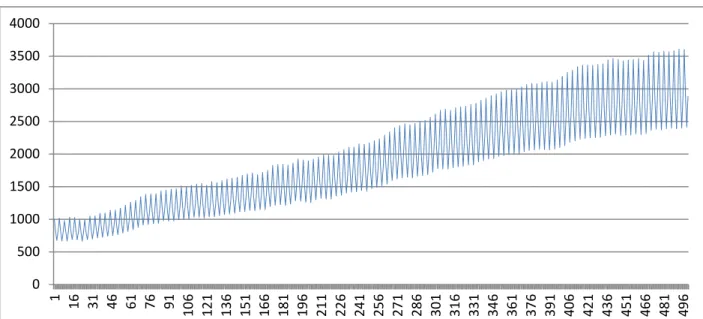
Finally we introduce our simulation results generating a so-called periodically integrated time series (see the figure below).⁴ The figure suggests estimating a multiplicative model as the seasonal swings grow in line with the trend. The characteristic of the prototype series of the Airline model is very similar.

Figure 1. Simulation results

Source: calculations of the author using GRETL

4 The simulated time series is the following: 𝑦_𝑡=𝑐+𝛼𝑠𝑦𝑡−1+𝜀𝑡, where the parameters are: 𝑐= 5, 𝛼1= 1.25, 𝛼₂= 0.80, 𝛼₃= 0.83, 𝛼₄= 1.20 (the product of the αs parameters is 1) and 𝜀_𝑡~𝑁(0.10) that is normally distributed random variable with mean of 0 and standard deviation of 10, and t = 1, 2 … 500. See the interpretation of the parameters in the following sections.

0 500 1000 1500 2000 2500 3000 3500 4000

1 16 31 46 61 76 91 106 121 136 151 166 181 196 211 226 241 256 271 286 301 316 331 346 361 376 391 406 421 436 451 466 481 496

(4)

We introduce the results applying the differencing filter (1− 𝐿)(1− 𝐿⁴) on a correlogram (see Figure 2). The problem of overdifferencing can be seen: some of the (partial) autocorrelation coefficients (PAC) significantly differ from zero.

Figure 2. Correlogram (PAC function) of the filtered time series: the results of applying differencing filter (1−L)(1−L⁴)

It is worth analyzing the effects of applying the seasonal differencing filter (𝟏 − 𝐋^𝟒). The (partial) autocorrelation coefficients display a non-elapsing sinusoid structure, so the polynominal does not filter the seasonal behaviour perfectly.

Figure 3. Correlogram (PAC function) of the filtered time series: the result of applying differencing filter (1−L⁴)

Naturally there are a lot of other transformations for filtering of trend and seasonality (e.g. incorporating different order of seasonal lags or seasonal dummy variables in the model). We cannot introduce all misspecifications in this paper, so we focus on the most frequent cases that were shown before.

Applying the periodic differencing filter (𝟏 − 𝛂_𝐬𝐋) as the suitable one, the filtered series is white noise (Figure 4). See the details in the following sections.

Figure 4. Correlogram (PAC function) of the time series: the results of applying periodic differencing filter (1− α_sL)

3. T HE STYLIZED FACTS OF ENERGY MARKETS

Stylized facts are (qualitative) characteristics of a homogeneous group of time series, which are independent of regional or temporal features. In the special case of energy markets the stylized facts are briefly the followings:

- time-dependent mean and variance,

(5)

- multiple seasonality,

- spikes and mean reversion in the case of price series.

The main source of time-dependent mean and variance are trend and seasonality. Time series often display a time-varying variance, see the higher volatility of power prices in summer and the higher volatility of consumption in spring and autumn. Seasonality on the other hand is multiple: depending on the granuality and the time series characteristics, we have to deal with yearly, weekly and daily seasonality. That means this feature displays in the long, medium and short run.

It is worth discussing price spikes and the short-term behaviour of the almost immediate mean reversion characteristic (see e.g. Burger et al. 2004). First we must mention that there is no correct and widely accepted definition of spikes in the literature, although there are a lot of references to cite. Some say that spikes are extrem values but they are inherently part of the series (see e.g. Burger et al. 2004 or Marossy 2010), while others say that spikes are outliers which must be replaced by normal values before taking any modelling steps. Spikes undoubtly make analysis more complicated (e.g. time series decomposition) and on the other hand they can lead to misspecifications as they can mislead standard test statistics (see for example testing for unit root in the presence of structural breaks in Mák 2011). It is clear that modelling spikes is a core component when dealing with time series with higher granuality (e.g. daily, hourly, quarterhourly). The reason we neglect spikes is that we place the emphasis on the long-term behaviour of time series such as the trend and annual seasonality and their interrelated evolution.

4. T RADING VOLUME AND LIQUIDITY IN THE E UROPEAN ENERGY MARKETS

In this section we briefly summarize the tendencies relevant from our paper’s point of view. The liquidity of energy markets – especially in the continental Europe – is far away from the liquidity experienced in the financial markets.⁵ The reasoning is partly historical (most of the markets are in their early years especially in the continental Europe), partly industry specific (spot trading means “bundled” physical and financial trading, while futures trading means only financial trading). The goals of future trading are mainly hedging, managing long-term risks, while the goals of spot trading is mainly portfolio (re)alignment and balancing.

Focusing on Europe, power and natural gas market development are highly different. Power markets came to focus as a result of the market coupling efforts, while natural gas markets are given more attention as a result of non-traditional sources (LNG, shale gas) and moving away from oil-indexed pricing of long-term contracts. The last one is one of the biggest questions of the future, but gas hubs seem to have a good opportunity to become the basis of pricing long-term contarcts. The Dutch hub TTF (Title Transfer Facility) has the largest chance of becoming the benchmark hub, although its trading volume is far behind the British NBP (National Balancing Point), but it is a good market place to handle volume and foreign exchange risk in comparison with NBP (energy unit of MWh vs. term and foreign exchange of EUR vs. GBP). The “trading profile” of other European hubs will likely be guided by portfolio alignment instead of determining wholesale price levels (see e.g. Heather 2012).

5. T IME SERIES ANALYZED IN THE PAPER

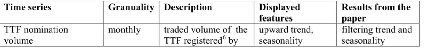
In this paper we analyze the time series specified in the following table:

Table 1. Time series analyzed in the paper Time series Granuality Description Displayed

features Results from the paper

TTF nomination

volume monthly traded volume of the

TTF registered⁶ by upward trend,

seasonality filtering trend and seasonality

5 The liquidity of energy markets can be measured by the bid-ask spread stemming from financial standards or by the so-called churn-rate which is the ratio between total volume of trade and the physical volume of trade, or the physical volume of gas consumed in the area served by the hub (see e.g. Heather 2012).

6 The traded volume registered by the „shippers” (for the sake of simplicity the traders) at the Dutch system operator on the network points. Nomination means ex ante demand announcement of natural gas for the following days or hours. The regulation of the nomination process (granuality, deadlines before physical delivery) can be different between countries.

(6)

the Dutch system

operator GTS⁷ influenced by heating effect EEX⁸ Phelix Day-

Ahead volume monthly volume of spot (day- ahead) trading in the EEX German and Austrian regions

slightly upward trend, “noisy”

seasonality

filtering trend and seasonality, capturing level shift

EEX Phelix Day-Ahead

price (average) monthly average price of spot (day-ahead) trading in the EEX German and Austrian regions

changing trend,

“noisy”

seasonality

filtering trend and seasonality, capturing level shift

Source: See data sources in Annex 1

See also the figures in Section 6 and Annex 1.Both the physical and financial volume of gas hubs have grown, while the trend in the case of power markets is not so clear. Seasonality is most remarkable in the case of natural gas (TTF) as a result of the so called winter or heating effect. Seasonality in the case of power is much more complex, see for example the effect of renewables on the within-a-day and day-ahead markets, the effects of natural gas and coal market movements on power markets and so on.

6. E MPIRICAL RESULTS

The detailed analysis of the periodic autoregressive (PAR) model and the periodic differencing filter are introduced on the example of the monthly nomination volume of TTF series. The main consequencies of modelling in the case of the other series are briefly summarized in the next section. The results were computed with the freely available R software packages. For detailed methodological issues see Annex 2.

6.1. A

NALYZING THE MONTHLY NOMINATION VOLUME OF THE

TTF

Figure 5 shows the monthly nomination volume of the TTF from January 2007. Data are available for earlier dates also but show the very unsystematic behaviour of the early trading activity on the TTF. The trading volume was much lower and seasonality less regular that time. It is worth mentioning that Hungarian consumption was around 12 and 14 million m³ in the last years, and we can see that in the years 2011, 2012 and 2013 the monthly trading volume on the TTF was far above this level almost every month.

Figure 5. Monthly nomination volume of the TTF [million m³]

Source: GTS, http://www.gasunietransportservices.nl

Besides the growing trend we can see that seasonal fluctuation grows in line with the trend, which suggests estimating a multiplicative model.⁹

7 Gasunie Transport Services

8 European Energy Exchange

9 Since the financial crisis of 2008, analyzing liquidity and its effect on price movements are very crucial issues.

Trading volume is of course insufficient to measure liquidity. Results analyzing trading volume, on the other hand, 0

5 000 10 000 15 000 20 000 25 000 30 000

2007M01 2007M05 2007M09 2008M01 2008M05 2008M09 2009M01 2009M05 2009M09 2010M01 2010M05 2010M09 2011M01 2011M05 2011M09 2012M01 2012M05 2012M09 2013M01 2013M05

(7)

6.1.1.MODEL SELECTION AND TESTING FOR UNIT ROOT

First we estimate a periodic autoregressive model of order p with intercept, i.e. the following:

𝑦𝑡,𝑠=𝑐+𝛷1,𝑠𝑦𝑡−1+𝛷2,𝑠𝑦𝑡−2+⋯+𝛷𝑝,𝑠𝑦𝑡−𝑝+𝜀𝑡 (1)

where 𝜀_𝑡 is white noise and s=1, 2 … 12. We can see that the autoregressive parameters are seasonally (or periodically) varying.

We estimate a model of order 1. The selection criteria are controversial but estimating with 2 lags means 12 additional parameters, which decreases the degree of freedom of the model so it is not proposed.

The F tests used are a Wald type tests that compares the models of order p and order 𝑝+ 1. When the restriction in the null hypotheses regarding the autoregressive parameters of order 𝑝+ 1 (i.e. all equal zero) does not significantly decreases the goodness of fit, it is not proposed to include the autoregressive variables of order 𝑝+ 1 in the model (that is 12 variables in our case). As the p-value to test the choice between the model of order 1 and 2 is 0.166, the null hypothesis cannot be rejected, therefore the model of order 1 is preferred.

After defining the PAR model of the specified order, we can check for periodicity in the autoregressive parameters of the model. The corresponding F test is again a Wald type F test. The restriction of the null hypothesis, that the parameters of order 𝑝 are equal, corresponds with an AR(p) model, and the alternative hypothesis corresponds with a PAR(p) model with periodically varing autoregressive parameters. The results show that the periodicity of the parameters cannot be rejected (as the corresponding p-value of the F test computed is 0.000), so the PAR(1) model fits better than an AR(1) model.

Testing for the unit root in the above definied PAR(1) model is the next highlighted issue and is discussed in the following. The tests are similar to the usual unit root tests. The null hypothesis corresponds with the presence of unit root, while the alternative hypothesis corresponds with stationarity.

One of the tests (the second one in our output, see below) is similar to the well-known left-tailed Dickey- Fuller test, the other test (the first one in our output, see below) is a right-tailed LR test. The logic behind applying the LR test is based on the restriction of the product of the periodically varying autoregressive parameters, that is the null hypothesis corresponds with the product constrained to unity and the alternative hypothesis corresponds with the unconstrained product. When the restriction significantly decreases the goodness of fit, the null hypothesis has to be rejected.

LR-test: 0.10

5 and 10% critical values:

when seasonal intercepts are included: 9.24, 7.52.

when seasonal intercepts and trends are included: 12.96, 10.50.

𝑠𝑖𝑔𝑛(∏¹²_𝑠=1𝛼𝑠−1) ·𝐿𝑅¹^�² test: -0.31 5 and 10% critical values:

when seasonal intercepts are included: -2.86, -2.57.

when seasonal intercepts and trends are included: -3.41, -3.12.

Source: Estimates computed with R Software

According to the results above, the null hypothesis of unit root cannot be rejected, in other words the nomination volume of the TTF is not stationary.

The next step is checking for the type of unit root whether the constrained autoregressive parameters are equal to +1 or –1 (i.e. the unit root is a long run unit root or a seasonal unit root). The tests are Wald type F tests again with the null hypotheses of the above mentioned constaints (autoregressive parameters are equal to +1 or –1). In both cases the calculated p-values are 0.000, which means that the time series contains neither long run nor seasonal unit root. According to this it is periodically integrated and a periodically integrated autoregressive model (PIAR) can be fitted.¹⁰

Checking for the robustness of our results, it is worth repeating the calculations when both intercept and trend are included in the model which is the following:

are controversial, some suggest the long memory property of trading volume (e.g. Lobato – Velasco 2000), others suggest a deterministic trend (e.g. Darbar – Deb 1995).

10 In Annex 2 we generalize the unit root tests for models of higher order. In this section we only mention briefly that the general test restricts on αs parameters which are the Φ1,s autoregressive parameters in our special case of the model of order 1.

(8)

𝑦_𝑡,𝑠=𝑐+𝑏·𝑡+𝛷_1,𝑠𝑦_𝑡−1+𝛷_2,𝑠𝑦_𝑡−2+⋯ 𝛷_1,𝑠𝑦_𝑡−1+𝜀_𝑡 (2) where 𝜀_𝑡 is white noise and 𝑠= 1, 2, … 12.

Selecting the order of lags the results are similar, so fitting a PAR(1) model is suggested. Notice that the trend parameter is slightly significant. The results cannot reject the nullhypothesis of the unit root again:

LR-test: 5.93

𝑠𝑖𝑔𝑛(∏¹²_𝑠=1𝛼𝑠−1) ·𝐿𝑅¹^�² test: -2.44

Source: Estimates computed with R Software, the critical values are equal to the ones in the previous case The following F tests suggest fitting a periodically integrated autoregressive (PIAR) model likewise. To decide whether a trend with constant or periodically varying parameters, and an intercept with constant or periodically varying parameters is needed, we can use Wald type F tests as usual. Without describing details we can say that the results stand for constant trend and intercept parameters. See Annex 2 for more details.

6.1.2.ANALYZING THE FINAL PIAR MODEL FOR THE NOMINATION VOLUME OF THE TTF As the results of the former section a PIAR(1) model with intercept is suggested. The model is the following (the 𝛼_𝑠 parameters are the autoregressive parameters, see Annex 2 for details):

𝑦_𝑡− 𝛼_𝑠𝑦_𝑡−1=𝑐+𝜀_𝑡 , (3)

or 𝑦_𝑡 =𝑐+𝛼_𝑠𝑦_𝑡−1+𝜀_𝑡, (4)

where 𝜀_𝑡 is white noise, 𝑠 = 1, 2 … 12, and the product of the seasonally varying 𝛼_𝑠 parameters is constrained to unity. We can see the parameter estimates and the corresponding p-values of the t type tests in the following table.

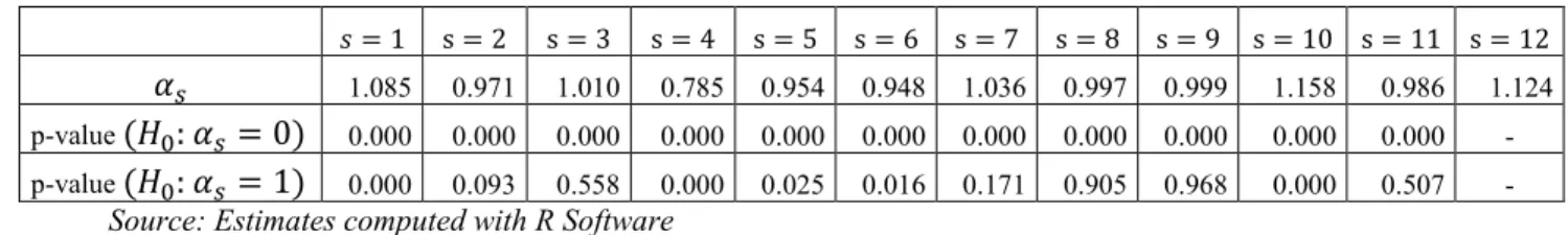
Table 2. Parameters and their significance levels in the PIAR(1) model

𝑠= 1 s = 2 s = 3 s = 4 s = 5 s = 6 s = 7 s = 8 s = 9 s = 10 s = 11 s = 12

𝛼_𝑠 1.085 0.971 1.010 0.785 0.954 0.948 1.036 0.997 0.999 1.158 0.986 1.124 p-value (𝐻0: 𝛼𝑠= 0) 0.000 0.000 0.000 0.000 0.000 0.000 0.000 0.000 0.000 0.000 0.000 - p-value (𝐻₀: 𝛼_𝑠= 1)^0.000 0.093 0.558 0.000 0.025 0.016 0.171 0.905 0.968 0.000 0.507 -

As we can see, all parameters are significant (𝐻₀: 𝛼_𝑠 = 0). It is even more interesting that most of them (January, April, May, June and October) significantly differ from unity. This is an empirical justification of seasonally varying parameters.

The matrix representation of the model helps us find how the stochastic trend and the seasonal fluctuations are related, in other words the following: which season has the highest long-term impact?

Which season undergoes the most severe impacts from the accumulation of shocks? See Annex 2 for more details about the computed matrices. The row and column with grey background contains sums of column and row elements.

Table 3: Time varying accumulation of shocks

1.000 1.030 1.020 1.298 1.361 1.436 1.386 1.390 1.391 1.201 1.218 1.085 14.816 0.971 1.000 0.990 1.260 1.322 1.394 1.346 1.350 1.350 1.166 1.183 1.053 14.385 0.981 1.010 1.000 1.273 1.335 1.408 1.360 1.363 1.364 1.178 1.195 1.064 14.531 0.770 0.793 0.785 1.000 1.049 1.106 1.068 1.071 1.071 0.925 0.939 0.836 11.413 0.735 0.757 0.749 0.954 1.000 1.055 1.018 1.021 1.022 0.882 0.895 0.797 10.885 0.696 0.717 0.710 0.904 0.948 1.000 0.965 0.968 0.969 0.836 0.848 0.755 10.316 0.721 0.743 0.736 0.936 0.982 1.036 1.000 1.003 1.003 0.866 0.879 0.783 10.688 0.719 0.741 0.734 0.934 0.979 1.033 0.997 1.000 1.001 0.864 0.877 0.781 10.660 0.719 0.740 0.733 0.933 0.979 1.033 0.997 0.999 1.000 0.864 0.876 0.780 10.653

(9)

0.833 0.857 0.849 1.081 1.133 1.196 1.154 1.157 1.158 1.000 1.014 0.903 12.335 0.821 0.845 0.837 1.065 1.117 1.179 1.138 1.141 1.141 0.986 1.000 0.890 12.160 0.922 0.949 0.940 1.197 1.255 1.324 1.278 1.281 1.282 1.107 1.123 1.000 13.658 9.888 10.182 10.083 12.835 13.460 14.200 13.707 13.744 13.752 11.875 12.047 10.727 -

Details of the impact matrix are the following (just examples, numbers in bold):

- 1,085 = the effect of a shock in December to January: 1,085 (𝛼₁₂)

- 1,053 = the effect of a shock in December to February: 1,085 · 0,971 (𝛼₁₂·𝛼₁)

- 0,164 = the effect of a shock in December to March: 1,085 · 0,971 · 1,010 (𝛼₁₂·𝛼1·𝛼2) - 1,195 = the effect of a shock in November to March: 1,124 · 1,085 · 0,971 · 1,010 (𝛼₁₁·𝛼₁₂·

𝛼₁·𝛼₂)

We can see that the effects can be calculated from the corresponding autoregressive parameters. The values of the sums of the column elements are higher from April to August, so these months have a higher long run impact. The values of the sums of the row elements are higher from October to March, so these months undergo a more severe impact from the accumulation of shocks. In other words the shocks in summer time swing the level of trading volume harder, while the shocks are more likely to accumulate in winter when the so-called heating effect holds.

6.1.3.APPLYING THE PERIODICALLY VARYING DIFFERENCING POLYNOMIAL

We complete the modelling of the TTF with applying more differencing filters on the time series. The usual first-order (non-seasonal) and seasonal differencing filters and the so-called periodic differencing filter resulting from the PIAR model estimates are computed. This latter filter is the following: (1− 𝛼_𝑠𝐿), where the αs parameters are the corresponding parameters in the PIAR model.

See Figure 6 for analyzing how the different filters performe.

Figure 6: Differencing filters applied on the nomination volume of the TTF [million m3]

Source: prepared by the author using estimates computed with R software

As we can see the seasonal differencing filter (i.e.(1−L¹²), thin line) filtered the seasonal variation and partly the growing trend. Checking for stationarity the correlogram shows that this series is stationary. So we misspecify when applying the first-oder differencing filter (i.e.(1− 𝐿)(1−L¹²), dotted line).Applying the so-called periodically varying differencing filter (i.e.(1− 𝛼_𝑠𝐿), bold line), the filtered series is smoother than the other two and contains fewer extreme values.

Checking for overdifferencing is hard as the series is quite short, and the filtered series – that is after applying (1− 𝐿)(1−L¹²) and (1− 𝛼𝑠𝐿) – seems to be quite similar. The conclusion supports the assumptions instead. Allowing the correlation of stochastic trend and seasonality can be ex ante justified (see the figure of the nomination volume of the TTF).

7. A DDITIONAL MODELLING RESULTS AND CONCLUSIONS

-4 000 -2 000 0 2 000 4 000 6 000 8 000

(10)

The above detailed analysis was repeated also on the other time series analyzed in the paper. The table below summarizes the main conclusions regarding the most suitable model variation.

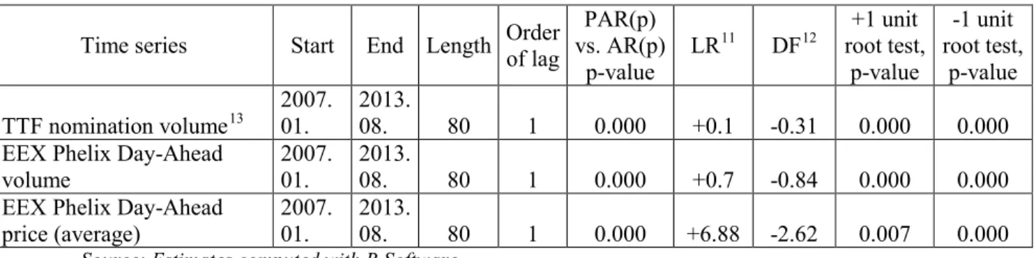
Table 4. Results on the other time series analyzed in the paper

Time series Start End Length Order of lag

PAR(p) vs. AR(p)

p-value LR¹¹ DF¹² +1 unit root test,

p-value

-1 unit root test,

p-value TTF nomination volume¹³ 2007.

01. 2013.

08. 80 1 0.000 +0.1 -0.31 0.000 0.000

volume 2007.

01. 2013.

08. 80 1 0.000 +0.7 -0.84 0.000 0.000

price (average) 2007.

01. 2013.

08. 80 1 0.000 +6.88 -2.62 0.007 0.000 Source: Estimates computed with R Software

It is worth underlining that the deterministic trend was not significant in neither of the models. Testing for the type of unit root, all tests suggest that the series can be modelled as periodically integrated autoregressive (PIAR) models.

Finally we introduce the filtered series after applying the three differencing filters as we did in the case of TTF. Applying the seasonal differencing filter on the trading volume of EEX, we can see that the trend has been filtered but the differencing filter did not handle the level shift in the year 2010. The sudden level shift also exists when we apply the periodic differencing filter. It seems to be useful to handle this event with an outlier dummy variable. On the other hand, we can see that applying the first-order differencing filter after the seasonal one, the filtered series contains more extreme values than in the case of the periodically differenced series. Results are similar in the case of the average price of spot trading in the EEX.

Figure 7. Differencing filters applied on the volume of spot (day-ahead) trading in the EEX [MWh]

Figure 8. Differencing filters applied on the average price of spot (day-ahead) trading in the EEX [EUR/MWh]

11 LR test, 5 and 10% critical values:

when seasonal intercepts are included: 9.24, 7.52.

when seasonal intercepts and trends are included: 12.96, 10.50.

12 𝑠𝑖𝑔𝑛(∏¹²_𝑠=1𝛼_𝑠−1) ·𝐿𝑅¹^�² test, 5 and 10% critical values:

when seasonal intercepts are included: -2.86, -2.57.

when seasonal intercepts and trend are included: -3.41, -3.12.

13 See details in Section 6.

-8 000 000 -6 000 000 -4 000 000 -2 000 000 0 2 000 000 4 000 000 6 000 000 8 000 000 10 000 000 12 000 000

(11)

Our results show that applying the periodic differencing filter results generally in smoother (with less outliers) and simpler time series in comparinson with other differencing filters, when the multiplicative assumption holds. The expression “simpler” means that the filtered series can be modelled with fewer lags in comparison with applying the other differencing polynomials. Note that the main conclusion is not the “simpler” differenced time series, but estimating the model with suitable assumptions.

We have to remark that applying the periodic differencing filter is not as general as other filters, as it uses the estimed parameters of the periodic autoregressive model directly. The filtered series also differs from the filtered results of the usual methods as trend and seasonalyity are filtered in one step.

-60 -40 -20 0 20 40 60 80

(12)

A NNEX 1: F IGURES OF OTHER TIME SERIES EXAMINED IN THE PAPER

Figure A1. Monthly volume of spot (day-ahead) trading in the EEX [MWh]

Source: www.eex.com (Regional Centre for Energy Policy Research)

Figure A2. Monthly average price of spot (day-ahead) trading in the EEX [EUR/MWh]

Source: www.eex.com (Regional Centre for Energy Policy Research) 5 000 0000

10 000 000 15 000 000 20 000 000 25 000 000 30 000 000 35 000 000 40 000 000

2007M01 2007M08 2008M03 2008M10 2009M05 2009M12 2010M07 2011M02 2011M09 2012M04 2012M11 2013M06

0 20 40 60 80 100

2007M01 2007M06 2007M11 2008M04 2008M09 2009M02 2009M07 2009M12 2010M05 2010M10 2011M03 2011M08 2012M01 2012M06 2012M11 2013M04

(13)

A NNEX 2: M ETHODOLOGICAL REVIEW

The goal of this section is to introduce the periodic autoregressive (PAR) model applied in the paper. This methodological overview is organised as follows. Section A2.1. discribes the periodic autoregressive (PAR) model, notations and interpretation. Section A2.2. discribes the main possible model selection steps (lag order, periodicity, including exogenous variables), while Section A2.3. introduces how to test for unit root. Finally (Section A2.4.) we show some theoretical background for interpreting the estimation results.

All the formulas in Annex 2 are presented for quarterly observed time series.

A2.1. T

HE PERIODIC AUTOREGRESSIVE

(PAR)

MODEL The well-known representation of an AR(p) model is as follows:

𝑦_𝑡 =𝛷₁𝑦_𝑡−1+𝛷₂𝑦_𝑡−2+⋯ 𝛷_𝑝𝑦_𝑡−𝑝+𝜀_𝑡, (A1)

where εt is a white noise process.

The so-called univariate representation of a PAR(p) model is as follows:

𝑦𝑡,𝑠=𝛷1,𝑠𝑦𝑡−1+𝛷2,𝑠𝑦𝑡−2+⋯ 𝛷𝑝,𝑠𝑦𝑡−𝑝+𝜀𝑡, (A2) where εt is a white noise process, 𝑠 = 1, 2, 3, 4, hence the autoregressive parameters vary with the season for each order of lag.

The process can be written by using the interaction of the corresponding seasonal dummy variable and lagged variable as follows (see e.g. Franses – Paap 1996):

𝑦𝑡 =∑ �𝛷4 1,𝑠(𝐷_𝑠∗ 𝑦𝑡−1) +𝛷2,𝑠(𝐷_𝑠∗ 𝑦𝑡−2)+. . +𝛷𝑝,𝑠�𝐷𝑠∗ 𝑦𝑡−𝑝��+𝜀𝑡

𝑠=1 , (A3)

where Ds variables are seasonally varying dummy variables and εt is a white noise process. That means the equation can be estimated by ordinary least squares. The empirical evidence behind applying seasonally varying parameters are that periodic autoregression allows for the presence of the interrelated stochastic trend and seasonality. In addition, in a lot of cases observations on a variable in some seasons have more impact on the dynamic pattern of the variable than observations in others seasons. Rougly speaking we can state that the effect of e.g. the first quarter of one year to the second is different from the effect of e.g.

the second quarter of one year to the third.

It is valuable to rewrite the univariate representation to a multivariate representation (vector of quarters representation or matrix representation), where the quarterly observed yt observations are stacked in the annually observed vector 𝑌_𝑇,𝑠=�𝑦_𝑇,1 𝑦_𝑇,2 𝑦_𝑇,3 𝑦_𝑇,4� that is the number of elements of the vector equals to the number of seasons. Note that the quarterly observed 𝑦_𝑡 and 𝑦_𝑇,𝑠 are the same, only the notation is changed: 𝑦_𝑡corresponds an observation in t (which is a quarter), 𝑦_𝑇,𝑠 corresponds an observation in year T and in quarter s. The advantage of the last notation is that we can explicitly indicate which quarters affects the values of other quarters. Going on with the above mentioned notation, the vector of quarters representation is as follows,

𝛷₀𝑌_𝑇,𝑠=𝛷₁𝑌_{𝑇−1,𝑠}+𝛷₂𝑌_{𝑇−2,𝑠}+⋯+𝛷_𝑝𝑌_{𝑇−𝑝,𝑠}+𝛦_𝑇, (A4) where

Ε

_T is a stacked white noise that is 𝛦_𝑇,𝑠 =�𝜀_𝑇,1 𝜀_𝑇,2 𝜀_𝑇,3 𝜀_𝑇,4� and 𝑠 = 1, 2, 3, 4.

For the sake of simplicity suppose that the order of lag needed for the quarterly observed series is 1, so the model is the following:

𝛷0𝑌𝑇,𝑠=𝛷1𝑌𝑇−1,𝑠+𝛦𝑇. (A5)

The annually observed stacked variables are

𝑌𝑇,𝑠 =�𝑦𝑇,1 𝑦𝑇,2 𝑦𝑇,3 𝑦𝑇,4� and

𝑌_{𝑇−1,𝑠}=�𝑦_𝑇−1,1 𝑦_𝑇−1,2 𝑦_𝑇−1,3 𝑦_𝑇−1,4�. (A6) The corresponding matrices are:

(14)

1,2

0 1,3

1,4

1 0 0 0

1 0 0

0 1 0

0 0 1

 

−φ 

 

Φ = −φ 

 −φ 

 

,

1,1

1

0 0 0 0 0 0 0 0 0 0 0 0 0 0 0

 φ 

 

Φ = 

 

 

, (A7)

and the reconstructed equations are as follows:

𝑦𝑇,1=𝛷1,1𝑦𝑇−1,4+𝜀𝑇,1

𝑦_𝑇,2 =𝛷_1,2𝑦_𝑇,1+𝜀_𝑇,2 𝑦_𝑇,3 =𝛷_1,3𝑦_𝑇,2+𝜀_𝑇,3 𝑦𝑇,4 =𝛷1,4𝑦𝑇,3+𝜀𝑇,4

(A8)

As we have seen, there can be three representations of the same periodic autoregressive model. A2 is useful for an easy interpretation, A3 is useful for the introduction of the estimation method. The A4 vector of quarters represenation might be strange and misleading as we have only one variable, so we conduct an univariate modeling and we also use a univariate estimation method. The vector of quarters representation is plausible as the result of periodically varying parameters and some tests (e.g. testing for unit root) and other results can only be accomplished through the use of this representation.

A2.2. M

ODELSELECTION

The first step we have to make is the selection of the order of the periodic autoregressive (PAR) model.

The formal selection can be based on the traditional Wald type F test. Under the nullhypothesis we make the restriction on the parameters of order 𝑝+ 1 are equal to zero against the alternative hypothesis that at least one of the parameters of order 𝑝+ 1 is significantly different from zero. The well-known selection criteria (e.g. Bayes Information Criteria, Akaike Information Criteria , adjusted R²) can be also applied.

The next step is to check whether seasonally varying autoregressive parameters are needed. The test is again a traditional Wald type F test. Under the nullhypothesis we make the restriction on the equality of the parameters from the same order, so an autoregressive (AR) model of order p is appropriate. Under the alternative hypothesis we allow the parameters from the same order to differ from season to season, so a periodic autoregressive (PAR) model fits better.

Behind the autoregressive variables, other variables can also be included in the model e. g. intercept and trend or seasonal dummy variables. Intercept and trend parameters can be constant or periodically varying. Finally, any periodic autoregressive model can be enlarged by exogenous variables. In the case of energy volume or price series these variables can be e.g. temperature, outlier dummies or dummies indicating holidays. Testing for significance can be performed in the tradional way (t tests and F tests).

A2.3. T

ESTING FOR UNIT ROOT

As we mentioned in the previous sections, it is often the case that stochastic trend and seasonality do not evolve independently and neither of the unit roots (non-seasonal or seasonal) exits on its own. In this case applying the seasonal differencing operator is not an appropriate solution. Periodic integration means that the autoregressive parameters can differ from unity either downward or upward, but their effect on the time series is equal to unity on the yearly average. The appropriate differencing operator also varies from season to season that is called the periodically varing filter or periodic differencing filter. That is why the periodic autoregressive model is appropriate. Testing for unit root means a two-step method in this case.

A2.3.1.TESTING FOR THE PRESENCE OF UNIT ROOT

Following the relevant references (e.g. Boswijk – Franses 1996) we first introduce testing for unit root in a model of order 1. The periodic autoregressive model of order 1 is as follows:

𝑦_𝑡 =𝛷_1,𝑠𝑦_𝑡−1+𝜀_𝑡, (A9)

where εt white noise and s = 1, 2, 3, 4. The corresponding vector of quarters representation is as follows:

𝛷0𝑌𝑇,𝑠=𝛷1𝑌𝑇−1,𝑠+𝛦𝑇, (A10)

(15)

where the matrices are known from (A7).

The vector process 𝑌_𝑇,𝑠 is stationary, if the roots of the characteristic equation (see (A11)) are outside the unit circle, see as follows:

|𝛷₀− 𝛷₁𝑧| = 0. (A11)

Computing the determinant above, the result is as follows:

�1− 𝛷_1,1𝛷_1,2𝛷_1,3𝛷_1,4𝑧�= 0. (A12)

We can see that the equation can have maximum 1 unit root, so checking whether the unit root exists means testing the following null hypothesis:

H0: 𝛷_1,1𝛷1,2𝛷1,3𝛷1,4=∏4 𝛷1,𝑠 𝑠=1 = 1, against the alternative hypothesis:

H1: 𝛷_1,1𝛷_1,2𝛷_1,3𝛷_1,4=∏⁴_𝑠=1𝛷_1,𝑠 < 1. (A13) To put it in other words, not rejecting the null hypothesis (when the root is on the unit circle) means that the time series is periodically integrated, rejecting the null hypothesis (when the root is outside the unit circle) means that the time series is periodically stationary. We often use the expression

‘stationary’ in brief, but note that the correct expression is ‘periodically stationary’, so stationary does not strictly hold as the autocovariances are time (season) dependent.

The equation to estimate is as follows:

𝑦_𝑡 =∑⁴_𝑠=1𝛷_1,𝑠𝐷_𝑠𝑦_𝑡−1+𝜀_𝑡, (A14)

and imposing the restriction under the nullhypothesis (A13), the restricted model is as follows:

𝑦_𝑡 =𝛷_1,1𝐷₁𝑦_𝑡−1+𝛷_1,2𝐷₂𝑦_𝑡−1+𝛷_1,3𝐷₃𝑦_𝑡−1+ (𝛷_1,1𝛷_1,2𝛷_1,3)⁻¹𝐷₄𝑦_𝑡−1+𝜀_𝑡, (A15) which we estimate using non-linear least squares.

As we make a nonlinear restriction on the Φ1,s parameters of the model, the (A13) hypotheses can be checked with the use of an LR (Likelihood Ratio) test. In the case, when the residual sum of squares does not reduce significantly as a result of the restriction, the null hypothesis can not be rejected (see Boswijk – Franses 1996; Franses 1996).

Another test which can be applied to test for unit root is introduced by Boswijk and Franses (1996) (the so-called 𝑠𝑖𝑔𝑛(∏¹²_𝑠=1𝛼𝑠−1) ·𝐿𝑅¹^�² test calculated from the LR test), who proved that the distribution of the test under the nullhypothesis of (A13) follows standard Dickey-Fuller. Enlarging the regression with intercept and trend, the corresponding Dickey-Fuller distribution can be applied (see Fuller 1976; Boswijk – Franses 1996).¹⁴

In the case of a periodic autoregressive model of order 2, the model is as follows:

𝑦_𝑡 =𝛷_1,𝑠𝑦_𝑡−1+𝛷_2,𝑠𝑦_𝑡−2+𝜀_𝑡 (A16)

where εt is white noise, 𝑠 = 1, 2, 3, 4 as before.

We can rewrite the (A16) model, that is:

𝑦_𝑡− 𝛼_𝑠𝑦_𝑡−1=𝛽_𝑠(𝑦_𝑡−1− 𝛼_𝑠𝑦_𝑡−2) +𝜀_𝑡 (A17)

and the characteristic equation can be written as follows (see Boswijk – Franses 1996):

|𝛷₀− 𝛷₁𝑧| = (1− 𝛼₁𝛼₂𝛼₃𝛼₄𝑧)(1− 𝛽₁𝛽₂𝛽₃𝛽₄𝑧) (A18) The corresponding hypotheses are:

H0: 𝛼₁𝛼₂𝛼₃𝛼₄=∏⁴_𝑠=1𝛼_𝑠= 1

14 We sould make a short notate that the distribution of the above mentioned LR test is not standard

χ

² distribution (see e.g. Boswijk–Franses (1996) and Osterwald-Lenum (1992) for details).

(16)

and H1: 𝛼₁𝛼2𝛼3𝛼4=∏4 𝛼𝑠

𝑠=1 < 1 (A19)

This means that under the null hypothesis we check whether the unit root exists, which corresponds with checking whether 𝛼₁𝛼2𝛼3𝛼4=∏4 𝛼𝑠

𝑠=1 = 1.

The model can be estimated with nonlinear least squares. Just a short note about βs parameters.

When we have a periodic autoregressive model of order 1, the βs parameters are all equal to zero. The above introduced (A17) model can be generalized for higher orders, but emprical results show that models with higher order than 2 are only sometimes needed.¹⁵

A2.3.2.TESTING FOR THE TYPE OF UNIT ROOT

When the null hypothesis of unit root cannot be rejected, we have to check for the type of the unit root.

The restriction of 𝛼₁𝛼₂𝛼₃𝛼₄=∏⁴_𝑠=1𝛼_𝑠= 1 can be fulfilled in two special cases, when the parameters are equal to +1 or –1. According to this, the following linear restrictions have to be checked with Wald type F tests:

H0: 𝛼_𝑠= +1 (A20)

where 𝑠 = 1, 2, 3 (it entails either αs= +1), and

H0: 𝛼_𝑠=−1 (A21)

where 𝑠= 1, 2, 3 (it entails either α_s= – 1).

The logic of applying Wald type F test is the same as before, as we impose a linear restriction on the (A17) models that the parameters are equal to +1 or –1. The first restriction corresponds to a process containing long-term unit root, the second one corresponds to a process containing seasonal unit root.

If the time series can be modelled as a periodically integrated autoregressive model, the αs

parameters are the seasonally varing parameters that differ from season to season. However on yearly average their cumulative effect does not significantly differ from unity. These αs parameters are slightly similar to seasonal indeces which are commonly used in modelling seasonality when trend and seasonality do not evolve independently, therefore a multiplicative model is required. Note that this similarity is misleading and not valid, because the αs parameters multiply the previous quarter’s value instead of the trend value in the same quarter, in contradiction with the traditional definition of the seasonal indeces.

A2.4. I

NTERPRETATION OF THE RESULTS A2.4.1.TIME VARING ACCUMULATION OF SHOCKS

We introduce how the time varing accumulation of shocks can be analyzed by applying the vector of quarters representation. The results can be enlarged up to higher orders, but we introduce the results assuming a maximum order of lag 4. In this case our vector of quarters representation is the following:

𝑌𝑇,𝑠 =𝛷1𝑌𝑇−1,𝑠+𝛦𝑇 (A22)

The left multiplication of both sides with matrix 𝛷₀⁻¹ results in:

𝑌_𝑇,𝑠 =𝛷₀⁻¹𝛷₁𝑌_{𝑇−1,𝑠}+𝛷₀⁻¹𝛦_𝑇 (A23)

where it is worth to define the following matrix:

𝛤=𝛷₀⁻¹𝛷₁ (A24)

The Γ matrix represents the effects of accumulated shocks of the seasons from the prevoius year to the seasons of the actual year. Indirectly we have shown that the 𝛷₀⁻¹ matrix represents the effects of accumulated shocks of the seasons to the seasons of the same year. When an eigenvalue of the Γ matrix exists, we can say, that the time series contains unit root. Going forward, we can define the following matrix which describes the time varing accumulation of shocks:

15 The R package we used for computing the results only allows for estimating models up to order 2.

(17)

𝛤𝛷₀⁻¹=𝛷₀⁻¹𝛷₁𝛷₀⁻¹. (A25) In the following step we introduce the impact matrix 𝛷₀⁻¹𝛷1𝛷0−1 representing the time varing accumulation of shocks in the case when only one lag is needed (as in the case of A7). From the point of view of this paper the presence of unit root is a highlighted issue, that is why we introduce the impact matrix with imposing the restriction 𝛷_1,1𝛷_2,1𝛷_3,1𝛷_4,1= 1. After some computation the impact matrix is as follows:

1,1 3,1 4,1 1,1 4,1 1,1

2,1 1,1 2,1 4,1 1,1 2,1

1 1

0 1 0

2,1 3,1 3,1 1,1 2,1 3,1

2,1 3,1 4,1 3,1 4,1 4,1

1

− −

φ φ φ φ φ φ

 

 φ φ φ φ φ φ 

 

Φ Φ Φ =

 φ φ φ φ φ φ 

φ φ φ φ φ φ 

 _. _(A26)

As the diagonal elements are all equal to unity, we can conclude that the effect of any quarter of the previous year is unity to the same quarter of the current year.

Let us take the last column of the impact matrix. The coefficients show how a shock from the fourth quarter of the previous year accumulates to the first, second, third and fourth quarters of the current year:

the coefficients are the multplications of the corresponding autoregressive parameters, and – of course – the last element is equal to unity. The other columns can be analyzed likewise. Take for example the third column of the impact matrix. The coefficients show how a shock from the third quarter of the previous year accumulates to the the first and second quarters of the actual year and the fourth quarter of the previous year (the order in time is of course different).

We can similarly analyze how the shocks coming from different quarters of the previous and actual years accumulate to the same quarter. The fourth row of the impact matrix represents how the shocks from the first, second and third quarters of the current year and the fourth quarter of the previous year accumulates to the fourth quarter of the current year. The other rows of the impact matrix can be analyzed likewise.

So the A26 matrix is clearly representing the time varing accumulation of shocks. Consequently we can discover how the stochastic trend and seasonality are related.

A2.4.2.APPLYING THE PERIODIC DIFFERENCING FILTER

Turning back to the beginning, we can state that in the case when the periodically integrated autoregressive model cannot be rejected, the periodically varing difference filter has to be applyed. The formal notation is (1− 𝛼𝑠𝐿) where the αs parameters are the estimation results introduced before.

R ^EFERENCES

Boswijk, H. P. – Franses, P.H. (1996): Unit roots in periodic autorregressions. Journal of Time Series Analysis 17: 221-245.

Box, G. E. P. – Jenkins, G. M. (1970): Time Series Analysis: Forecasting and Control. San Francisco:

Holden Day.

Burger, M. – Klar, B. – Müller, A. – Schindlmayr, G. (2004): A spot market model for pricing derivatives in electricity markets. Journal of Quantitive Finance 4(1): 109-122.

Clements, M. P. – Hendry, D. F. (1997): An empirical study of seasonal unit roots in forecasting.

International Journal of Forecasting 13(3): 341-355.

Darbar, M. S. – Deb, P. (1995): Does trading volume have a unit root? Applied Economics Letters 2(5):

144-147.

Franses, P. H. (1996): Periodicity and Stochastic Trends In Economic Time Series. Oxford: Oxford University Press.

Franses, P. H. (1998): Time Series Models for Business and Economic Forecasting. Cambridge:

Cambridge University Press.

Franses, P. H. – Paap, R. (1996): Periodic integration: further results on model selection and forecasting.

Statistical Papers (37): 33-52.

Fuller, W. A. (1976): Introduction to Statistical Time Series. New York: Wiley.

Heather, P. (2012): Continental European Gas Hubs: Are they fit for purpose? Oxford Institute for Energy Studies.

Hylleberg, S. – Engle, R. F. – Granger, C. W. J. – Yoo, B. S. (1990): Seasonal Integration and Cointegration. Journal of Econometrics 44: 215-238.

(18)

Lieli, R. (1999): Az idősormodelleken alapuló inflációs előrejelzések: egyváltozós módszerek [Inflation Forecasts Based on Time Series Models – Single Variable Methods]. MNB füzetek 1999(4): 1-68.

Lobato, I. N. – Velasco, C. (2000): Long Memory in Stock-Market Trading Volume. Journal of Business and Economic Statistics 18(4): 410-427.

Mák, F. (2011): Egységgyöktesztek alkalmazása strukturális törések mellett a hazai benzinár példáján [Unit Root Tests with Structural Breaks – The Hungarian Example of Petrol Prices]. Statisztikai Szemle 89(5): 545-573.

Marossy, Z. (2010): A spot villamosenergia árak elemzése statisztikai és ökonofizikai eszközökkel [Analysis of spot electricity prices using statistical and econophysical methods]. Ph.D. dissertation, Corvinus University of Budapest

Osterwald-Lenum, M. (1992): A Note with Quantiles of the Asymptotic Distribution of the Maximum Likelihood Cointegration Rank Test Statistics: Four Cases. Oxford Bulletin of Economics and Statistics (54): 461-472.

Sugár, A. (1999a): Szezonális kiigazítási eljárások (I.) [Seasonal Adjusment Methods (I.)]. Statisztikai Szemle 77(9): 705-721.

Sugár, A. (1999b): Szezonális kiigazítási eljárások (II.) [Seasonal Adjustment Methods (II.)]. Statisztikai Szemle 77(10-11): 816-832.