PLANE SEGMENTATION FROM POINT CLOUDS 1

DOI: 10.1556/606.2018.13.2.16 Vol. 13, No. 2, pp. 159–171 (2018) www.akademiai.com

PLANE SEGMENTATION FROM POINT CLOUDS

1 Richard HONTI, ² Ján ERDÉLYI, ³ Alojz KOPÁČIK

1,2,3

Department of Surveying, Faculty of Civil Engineering

Slovak University of Technology in Bratislava, Radlinského 11, 810 05 Bratislava e-mail: ¹richard.honti@stuba.sk, ²jan.erdelyi@stuba.sk, ³ alojz.kopacik@stuba.sk

Received 7 December 2017; accepted 27 March 2018

Abstract: Recently, attempts have been made to automate data acquisition, which is also related to efforts to automate data processing. The paper deals with the automation of terrestrial laser scanning data processing. The approaches for point cloud segmentation are briefly described. An algorithm based on random sample consensus is proposed for automated plane identification and plane segmentation from point clouds. The proposed approach was tested by processing point clouds; the results of the testing are also described. Based on the proposed algorithm, a standalone application for automated plane segmentation from laser scanner data using Matlab^® software was developed.

Keywords: Terrestrial laser scanning, Point cloud, Plane segmentation, Automated data processing, Random sample consensus

1. Introduction

Terrestrial Laser Scanning (TLS) is becoming the main technique for the acquisition of spatial information in a variety of fields (e.g. the civil engineering, topographic, environmental, industrial and cultural heritage fields, etc.). High quality 3D models of objects have an important role in a variety of areas, e.g. interior (exterior) design, Building Information Modeling (BIM), urban information systems, documentation, 3D cadaster, etc. Due to the rapid development of scanning technologies, very large sets of 3D points of required accuracy can be collected easily and quickly. As a result of scanning, point clouds are becoming an increasingly common initial digital representation of real-world objects. This is due to the popularity of affordable and

accurate scanning equipment that can quickly digitize the geometry of a real-world object [1], [2], [3]. With the development of hardware, the processing of acquired data is gaining more and more attention. Therefore, development of data processing applications is also very important (e.g. [4], [5]), because to be able to use of data effectively, raw data has to be enriched to provide the user with a higher level of interactive possibilities.

To quickly derive higher levels of abstraction, primitive geometric shape detection is advisable [6]. Segmentation is a fundamental step in the processing of 3D point clouds.

Thanks to segmentation, geometric shapes from a point cloud can be selected. To increase the efficiency of 3D model creation from TLS data, automation of the processing steps is desirable. The automated segmentation of a point cloud helps with the processing and shortens the time needed for processing, especially when creating a 3D model. Since in most cases point clouds represent a huge amount of data, the efficiency of the processing algorithms is very important. Thus, this paper is focused on finding an efficient, robust, and accurate algorithm for automated point cloud plane detection. The algorithm is based on the Random Sample Consensus (RANSAC) [7]

paradigm, which is capable of extracting a variety of different types of primitive shapes, while retaining the leading properties of the RANSAC paradigm as robustness, generality, and simplicity. The algorithm developed is aimed at extracting planes automatically, efficiently and accurately from scanned data.

The paper presents a proposed method for automated TLS data processing for plane identification and segmentation. A standalone application for this purpose based on the proposed algorithm was developed. The benefits of the proposed method are demonstrated by the application of the derived method on data resulting from the scanning of an actual scenario.

The paper briefly introduces the TLS method, describes the segmentation process of TLS data, and describes the methods and approaches for point cloud segmentation. It then introduces the proposed algorithm for automated plane identification and segmentation. Since the algorithm is based on the RANSAC paradigm, the RANSAC algorithm is described along with the necessary changes for the practical use of RANSAC for plane segmentation. The paper further presents the testing and the experimental results from the testing of the proposed algorithm and describes the standalone application based on the proposed algorithm, which has been developed for automated plane segmentation using Matlab^® software.

2. Terrestrial laser scanning

The advantage of TLS is that it allows for non-contact documentation of the object measured with all its structural elements without the need to define some characteristic points on the surface of the object measured. The difference between TLS and conventional surveying methods is that the coordinates of the characteristic points are obtained by modeling the main elements of 3D models or the resulting point clouds [8], [9], [10].

The technology of TLS is a non-selective method of spatial data acquisition. TLS determines the 3D coordinates of the points measured on the surface of the object

measured in a grid, which is defined by regular angular spacing in the horizontal and vertical directions. The results of a measurement by TLS is an orderless set of measured 3D points, i.e. the so-called Point Cloud (PoC), (Fig. 1) [8].

Fig. 1. The result of a measurement - point cloud

Most contemporary TLS works on the principle of the spatial polar method. The spatial position of the points measured is calculated from the horizontal and vertical angles and the slope distance measured [8]. The scanning speed with current scanners reaches 1 million points per second, which means that the time needed for measuring an object is significantly reduced.

The process of determining the 3D position of an object measured using TLS can be divided into three main steps. The first step is the preparation for the measurement (recognition of the scanned object, the choice of instrument positions and signalization of the control points). The second step is the measuring (scanning) of the object and the third is the TLS data processing (modeling, segmentation, visualizations, graphs, etc.) [8].

3. Segmentation of point clouds

Processing point clouds and the consecutive creation of 3D models of objects measured are contemporary topics. The segmentation of point clouds is the process of classifying points of a point cloud into multiple homogeneous regions; the points in the same region will have the same properties. The most common segmentations of point clouds are those where group points fit onto the same plane, cylinder or other geometric primitive. The segmentation is then equivalent to the recognition of simple shapes in a point cloud. Because of the high amount of redundancy, uneven sampling density, and the absence of an explicit structure of point cloud data, segmentation can be challenging. In many cases the PoC contains missing parts as the result of covers (hidden parts of the object scanned) (Fig. 2); moreover, the scanned object can be somewhat rugged and consists of various complex geometric shapes [9], [11].

Fig. 2. Point cloud with missing parts

In the next section the methods and algorithms that have been suggested in [11] for 3D point cloud segmentation are briefly described. These methods could be generally categorized into 5 classes.

3.1. Edge-based methods

An edge describes the characteristics around the shape of an object. Edge-based methods are based on the detection of the boundaries of separate sections in a PoC to obtain some segmented regions. An edge detection technique was suggested by Bhanu et al. [12]. The principle of these methods is based on searching points, which shows a rapid change in the intensity, computing the gradient, fitting 3D lines to a set of points, and detecting changes in the direction of the unit normal vectors of the surface [11].

3.2. Region-based methods

Region-based methods use neighborhood information to merge close points that have identical properties to obtain segregated regions and consequently find dissimilarities between separate regions. Compared to the edge-based methods, region- based methods are less sensitive to noise, but they have a problem with over and under- segmentation and with correct detection of a region’s boundaries. The region-based methods can be divided into two categories: seeded-region methods [13] and unseeded- region methods [11].

3.3. Attributes-based methods

Attribute-based methods consist of two separate steps. The first step is computation of the attribute; in the second step, the PoC will be clustered based on the attributes computed. One limitation of these methods is that they are dependent on the quality of the attributes acquired [11], [14], [15].

3.4. Model-based methods

Model-based methods use geometric shapes (e.g. planes, spheres, cylinders, and cones) to organize points. The points, which have the same mathematical representation are grouped as one segment. A well-known algorithm called RANSAC was suggested by Fischer [7]. RANSAC is a robust model and can be used for the detection of geometric shapes (see Section 4.1). This method is now state-of-the-art for fitting models. Many works rely on this algorithm, e.g. [11].

3.5. Graph-based methods

Graph-based methods deal with the PoC in terms of a graph. These methods are precise and efficient; thus, they are popular for robotic applications [11]. Strom et al.

[16] extended a graph-based method to segment colored 3D laser data.

4. Automated plane segmentation using RANSAC 4.1. RANSAC

RANSAC is an iterative method for estimating a mathematical model from an observed data set, which contains outliers. The algorithm was first published in [7].

RANSAC works by identifying the outliers in a data set and estimating the desired model using data that does not contain outliers; therefore, the RANSAC paradigm extracts shapes from the point data and constructs corresponding primitive shapes, based on the notion of minimal sets. A minimal set is the smallest number of data samples required to uniquely define a model (e.g. three points for a plane, four for a sphere, etc.). The resulting candidate shapes are tested against all the points in the data to determine which points are well approximated by the primitive. After a given number of iterations, the shape which approximates the most points is extracted, and the algorithm continues with the remaining data [7], [6], [17].

A simple example of using RANSAC for line fitting in 2D to a set of measured points can be seen in Fig. 3. On the left side is the set of points, including the outliers.

The right side in the blue (asterisk) color shows the inliers for the line and the fitted line; the red (points) color shows the outliers, which, as is also shown in Fig. 3, do not affect the line fitting by RANSAC.

The advantage of RANSAC is its robust estimation of the unknown parameters of a model with a high level of accuracy, even in the presence of a high percentage of errors (outliers). The disadvantage is that if the data is sustainable for two or more models, the method may fail, and no model may be found [6]. The use of the RANSAC described for identifying and segmenting planes is not entirely proper and has some limitations, while in the case of fitting a plane, RANSAC starts with the selection of 3 neighboring points to a randomly selected seed point, approximates this neighborhood with an initial plane, and tests the other points if they are lying on the initial plane at a selected threshold number (most often, the distance to the plane).

Fig. 3. RANSAC [18]

In this procedure a cross-section of a closed scanned object may be selected (Fig. 4) so that in the testing process, only the points, which are lying in this cross-section would be added, so that it would already be failing to refine the calculations. In Fig. 4 the planes fitted by RANSAC are shown; it can be seen from this figure that these planes do not represent any of the characteristic planes of the scanned object. The next limitation is that in RANSAC, every data point has to be evaluated against the model, and every data point is evaluated individually; this is repeated for all iteration of the algorithm.

This procedure is quite time consuming.

Fig. 4. Point cloud with planes fitted by RANSAC

Due to the inapplicability of RANSAC, it was necessary to propose a modified algorithm, which eliminates these disadvantages. The modified algorithm is described in the next section.

4.2. RANSAC - a proposal for plane segmentation

The proposed algorithm (for plane segmentation from point clouds) is based on RANSAC, but it eliminates RANSAC’s limitations and disadvantages (see the previous

section). The algorithm also gradually accelerates, which is a very positive asset from the point of view of efficiency.

The algorithm starts at the beginning with selection of 10 (not 3, as in RANSAC) neighboring points to the seed point, which have been chosen (a non-random selection of seed points against RANSAC). The seed points for every plane are defined by its spatial coordinates. Then, this neighborhood is approximated by a plane. The estimation of the plane is done by orthogonal regression, which minimizes the perpendicular distances to the plane. The solution is based on the general equation of a plane:

0

= +

⋅ +

⋅ +

⋅X b Y c Z d

a , (1)

where a, b and c are the parameters of the normal vector of the plane; X,Y,Z are the coordinates of a point lying on the plane; and d is the scalar product of the normal vector of the plane and the position vector of any point of the plane. To calculate the elements of the normal vector, the Singular Value Decomposition (SVD) is used [19]:

VT Σ U

A = ⋅ ⋅ , (2)

where A is the design matrix with dimensions of n×3; n is the number of points used for the calculations. The column vectors of U are normalized eigenvectors of the matrix AA^T. The column vectors of V are normalized eigenvectors of A^TA. The matrix Σ contains eigenvalues on the diagonals. The normal vector of the regression plane is the column vector of V corresponding to the smallest eigenvalue from Σ. The plane is then defined by the elements of the normal vector a, b and c. Parameter d is calculated by fitting the elements of the normal vector and the coordinates of the centroid of the point cloud according to the formula

(

)

d=− ⋅ + ⋅ + ⋅ . (3)

The orthogonal distances of the points from the plane are calculated as follows:

( )

2 2

2 b c

a

d c b a p

+ +

+

⋅ +

⋅ +

= ⋅X Y Z

d _{. (4)}

In the next step the region is grown by clustering the points that are geometrically compatible with the approximated plane, i.e. from the 100 closest points, those are selected for which the value of d_p (4) is less than a selected threshold number, so they meet the distance criterion. Once all the compatible points have been added, the algorithm fits a new plane to the region to improve the approximation. The algorithm then uses this new plane to re-grow the region. Then, in the next step, 400 neighboring points are tested, then 1,600 neighboring points, then 6,400, etc. So, every iteration has four times more points for testing (using RANSAC, every randomly selected point is tested individually).

After each iteration, the plane is recalculated using all the points that meet the specified criterion. The criterion in this case is the distance of the points from the plane, e.g. at a 5 mm threshold number, only the points are used whose distance from the plane is less than 5 mm. The ‘region growing’ is repeated until the region’s size stops increasing.

The advantage of the proposed method is that the testing is always performed on the closest points, not on those randomly selected. The number of points for testing is increased four times, so that through the process of the algorithm the calculations are accelerating. The iterative increases and testing of only the closest points dramatically shortens the time needed for the calculations and overcomes the limitations of RANSAC as described in Section 4.1.

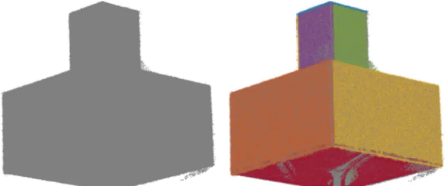
After completing the iterative enlargement, i.e. selecting all the points that belong to the given plane, these points are removed from the original point cloud; this means that while searching for the other planes, the testing is executed only on the remaining points (excluding the points which belong to a previously estimated plane). This step also significantly reduces the time required for the calculations. Fig. 5 shows a demonstration of the point cloud segmentation of the model figure (a double cube) through the use of the given algorithm, where different planes are color differentiated.

Fig. 5. Demonstration of the point cloud segmentation of a model figure original point cloud (left), segmented planes (right)

4.3. Software development

The proposed segmentation procedure places high demands on the computer used for data processing, as well as on the operator itself. For the automation of the above- mentioned procedure, a computational ‘PC_Segmentation’ application was developed (Fig. 6). The application is based on Matlab® software.

The application was created as a stand-alone application; however, Matlab®

Runtime is needed for its execution. The work with the application is done as follows:

The first step is loading the point cloud file in the *.txt or *.xyz file format that contains the spatial coordinates of the points scanned. The plane points can also be arranged in a

*.txt or *.xyz file that defines the coordinates of the seed points of the individual planes.

The segmentation process starts with the points defined by the mentioned file, and the

regions are grown from these points. Before starting the segmentation process, it is necessary to select the threshold number for estimating the plane. According to the results of the segmentation process, the individual point clouds for the estimated planes are saved into a *.txt file in a new folder called ‘Results’ in the work directory, and the plane parameters are shown in the ‘Plane parameters’ table on the right side of the application’s dialog window. The table contains the IDs of the planes, their estimated parameters (a, b, c, d), the number of compatible points of the planes, and the standard deviation of the planes estimated. A figure (Fig. 6, right), which shows the original point cloud and the separate point clouds for the estimated planes (various colors depict various planes), is created for the consistent monitoring of the application process, so the user can visually check whether the individual planes are correctly segmented. This figure can be saved in various file formats (i.e. *.tif, *.png, *.bmp, *.pdf, *.jpg, etc.).

Fig. 6. Dialog window of the application

The bottom side of the application’s dialog window serves for the execution of the plane’s recalculation. The user can choose a new threshold number and the planes which need recalculation.

5. Testing of the proposed algorithm

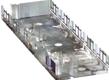
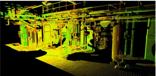
For the experimental testing of the above-described proposed algorithm, a point cloud of the Laboratory of Surveying (Faculty of Civil Engineering, STU in Bratislava) (Fig. 7) was used.

Fig. 7. Laboratory of Surveying

The process for the application described is shown in (Fig. 8 and Fig. 9). The figures show that, during the iterative region-growing process, the points selected for testing are not only those which are lying on the given plane, due to the fact the quadratic growth of the region is done spatially. These points are excluded during the testing, e.g. they do not affect the estimation of the plane at all. At the end, only the points that belong to the given plane (at a selected threshold number) are selected.

Fig. 8 shows the point cloud measured and the process of the iterative growth of the testing region. In right the selected seed point (in the center of the circles), and the 102,400 nearest points are shown, so the process of selecting the points for testing around the seed point selected. The iterative growth of the number of the points is illustrated by different colors: green (diamond) - 10; purple (plus sign) - 100; dark blue (downward-pointing triangle) - 400; black (circle) - 1,600; light blue (asterisk) - 6,400;

dark blue (square) - 25,600; yellow (right-pointing triangle) - 102,400 of testing points.

From Fig. 8 it is obvious that the region’s growth is performed spatially.

Fig. 8. Measured point cloud (left); gradually growing the region of the selected points around the seed point (center - 6,400 points, right - 102,400 points)

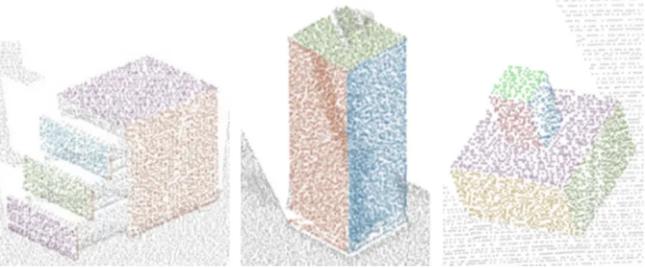
Fig. 9 shows the input point cloud; the blue color shows the points of the segmented plane at a 5 mm threshold number (the orthogonal distance of the points from the estimated plane). In Fig. 10 the details of the plane segmentation process are shown; the left side of the figure shows the individual planes of a bank; the center shows the individual planes of a pillar; and the right side shows the individual planes of a double cube.

Fig. 9. The estimated plane by the algorithm described

Fig. 10. Details of the segmentation result

Fig. 10 (left) shows the individual planes of a bank (part of the PoC of the laboratory scanned). The whole bank consists of approximately 25,500 points and 6 planes. The segmentation process was accomplished with a 5 mm threshold number (i.e.

the plane estimation was done based on the points which were closer, than 5 mm to the estimated plane). The standard deviation, calculated based on orthogonal distances of the points from the plane estimated, was less than 1.2 mm in any cases. According to the results, 6 planes were segmented with total of 23,385 points. That means approximately 2,115 points were not included in the segmentation process (the points not lying in the planes segmented, e.g. the pulls of the cabinet etc.), which represents just 8.29% of the total number of points. With the above described segmentation algorithm, extreme time reducing was achieved, because after a plane is segmented,

these points are excluded from the original point cloud, so by the process of the application there are fewer and fewer points for testing.

6. Conclusion

Automated 3D model creation is a topic of contemporary interest and is closely connected with automated point cloud processing, because point clouds obtained by TLS are currently one of the basic documents often used for 3D model creation. One of the most important steps of point cloud processing is the segmentation of various geometric shapes from the point cloud.

The paper briefly describes the methods and approaches for point cloud segmentation. A proposed algorithm for automated plane identification and segmentation from point clouds is described. The algorithm is based on RANSAC, but due to the inapplicability of RANSAC, some modifications were necessary. The modifications are described in this paper. The proposed algorithm was implemented as a stand-alone application. The user can easily execute the plane segmentation of point clouds with the application created. The results of the application are the segmented points saved into text files for every plane and the parameters of the segmented planes shown in the table of the application’s dialog window. The benefits of the proposed method for plane segmentation are the robust and accurate segmentation of point clouds, which can have an uneven density and contain noise. The parameters of the planes are calculated using SVD, which means that no initial parameters are needed for the data processing. The whole process takes only several minutes, as the calculations described in Section 4.2 are executed automatically for all the planes (approximately 850,000 points) represented by the seed points loaded.

Acknowledgements

This article was created with the support of the Ministry of Education, Science, Research and Sport of the Slovak Republic within the Research and Development Operational Programme for the project ‘University Science Park of STU Bratislava’, ITMS 26240220084, co-funded by the European Regional Development Fund.

References

[1] Berényi A. Laser scanning in engineering survey - An application study, Pollack Periodica, Vol. 5, No. 2, 2010, pp. 39‒48.

[2] Tran T. T., Cao V. T. Laurendeau D. Extraction of cylinders and estimation of their parameters from point clouds, Computers & Graphics, Vol. 46, 2015, pp. 345‒357.

[3] Vieira M., Shimada K. Surface extraction from point-sampled data through region growing, International Journal of CAD/CAM, Vol. 5, No. 1, 2005, pp. 19‒27.

[4] Molnár B. Developing a web based photogrammetry software using DLT, Pollack Periodica, Vol. 5, No. 2, 2010, pp. 49‒56.

[5] Somogyi Á., Lovas T., Barsi Á. Comparison of spatial reconstruction software packages using DSLR images, Pollack Periodica, Vol. 12, No. 2, 2017, pp. 17‒27.

[6] Schnabel R., Wahl R., Klein R. Efficient RANSAC for point-cloud shape detection, Computer Graphics Forum, Vol. 26, No. 2, 2007, pp. 214‒226.

[7] Fischler M. A., Bolles R. C. Random sample consensus: A paradigm for model fitting with applications to image analysis and automated cartography, Communications of ACM, Vol.

24, No. 6, 1981, pp. 381‒395.

[8] Erdélyi J., Kopáčik A., Kyrinovič P., Lipták I. Automation of point cloud processing to increase the deformation monitoring accuracy, Applied Geomatics, Vol. 9, No. 2, 2017, pp. 105‒113.

[9] Vosselman G., Maas H. G. (Eds) Airborn and terrestrial laser scanning, Dunbeath:

Whittles Publishing, 2010.

[10] Kašpar M., Pospíšil J., Štroner M., Křemen T., Tejkal M. Laser scanning in civil engineering and land surveying, Vega s.r.o., Hadec Králové, Czech Republic, 2004.

[11] Nguyen A., Le B. 3D point cloud segmentation: A survey, 6th IEEE Conference on Robotics, Automation and Mechatronics (RAM), Manila, Philippines, 12-15 November 2013, pp. 225‒230.

[12] Bhanu B., Lee S., Ho C. Henderson T. Range data processing: Representation of surfaces by edges, University of Utah, Department of Computer Science, 1985.

[13] Rusu R., Marton Z., Blodow N., Dolha M. Beetz M. Towards 3D point cloud based object maps for household enviroments, Robotics and Autonomous Systems, Vol. 56, No. 11, 2008, pp. 927‒941.

[14] Biosca J. M., Lerma J. L. Unsupervised robust planar segmentation of terrestrial laser scanner point clouds based on fuzzy clustering methods, ISPRS Journal of Photogrammetry and Remote Sensing, Vol. 63, No. 1, 2008, pp. 84‒98.

[15] Filin S. Surface clustering from airbone laser scanning data, in International Archives of Photogrammetry, Remote Sensing and Spatial Information Sciences, Vol. XXXII, No. 3A, 2002, pp. 117‒124.

[16] Strom J., Richardson A., Olson E. Graph based segmentation of coloured 3D laser point clouds, Proc. of the IEEE/RSJ International Conference on Intelligent Robots and Systems (IROS), Taipei, Taiwan, 18-22 October 2010, pp. 2131‒2136.

[17] Hampacher M., Štroner M. Processing and analysis of the data measured in engineering geodesy, (in Czech) Czech technical University in Prague, Czech Republic, 2011.

[18] RANSAC, Wikipedia, https://en.wikipedia.org/wiki/Random_sample _consensus, (last visited 30 October 2017).

[19] Čepek A., Pytel J. A note on numerical solution of least square adjustment in GNU Project Gama, In: Pilz J. (Ed.) Interfacing Geostatistics and GIS, Springer, Berlin, 2009.