Appropriate Mathematical Model of DC Servo Motors Applied in SCARA Robots
Attila L. Bencsik
Bánki Donát Faculty of Mechanical Engineering, Budapest Tech Népszínház utca 8, H-1081 Budapest, Hungary
bencsik.attila@bgk.bmf.hu
Abstract: In the first part of the presentation detailed description of the modular technical system built up of electric components and end-effectors is given. Each of these components was developed at different industrial companies separately. The particular mechatronic unit under consideration was constructed by the use of the appropriate mathematical model of these units. The aim of this presentation is to publish the results achieved by the use of a mathematical modeling technique invented and applied in the development of different mechatronic units as drives and actuators. The unified model describing the whole system was developed with the integration of the models valid to the particular components. In the phase of testing the models a program approximating typical realistic situations in terms of work-loads and physical state of the system during operation was developed and applied.
The main innovation here presented consists in integrating the conclusions of professional experiences the developers gained during their former R&D activity in different professional environments. The control system is constructed on the basis of classical methods, therefore the results of the model investigations can immediately be utilized by the developer of the whole complex system, which for instance may be an industrial robot.
Keywords: mechatronic, system investigation, industrial robot, DC servo motor, PID control
1 Model of the Servo Motor
The first step was to design the model of a PM motor in order to perform the analysis. The system model has two main parts and several smaller units.
Figure 1
Figure 2
As a following step the control circuit was developed using the previous results.
Ube( )t =URa +ULa +Ui (1)
Ube( )t =i Ra a+L di (2)
dt K
a a + 1
Ui =KiΩ (3)
Mmot −Mload" =Maccelerat d
or = Θ dtΩ
(4) K la M2 − load −BVΩ Θ= Ω
(5) d
dt Loop of the circle:
Ube( )t =ia −Ra +La di
dta +K1Ω (6)
K i d
a dt
2 =Θ Ω+
Mload+BVΩ (7)
The system-model:
L d m
dt U t
a a
be a
.
= ( )−i Ra−K1Ω (8)
ΘdΩ
dt =K i2 a−Mload+BVΩ (9)
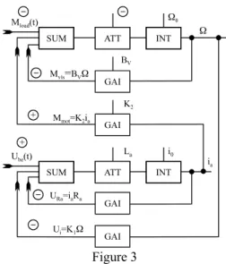
Figure 3 Interpretation of the blocks in system description
Out=In1+In2
Out In
= P Out=In P⋅
Out=
∫
In dt⋅ Motor given by the system-model can be regarded as only unitParameters of the motor used in simulation 80W Ra = 0,360 [W] La = 0.14.10-3 [H]
Qrotor = 1,22.10-4 [kg.m2] K1 = 50,1.10-3 [Vs]
Mn =0,301 [Nm]
K2 = 50,1.10-3 [Nm/A]
Ube = Un = 15 V
Bv clamping coefficient (viscosity) is not given in the cataloge. Let take the value of Bv so that in slow running, no-load current flows in the motor, I0 = 324 mA.
W0 = 286,78 rad/s. If I0 = 310 mA then Mvis = 0,05.Mn ! Then Bv = (0,05.Mn)/W0 = 5,23.10-5 [Nms]
Time constants of the motor: T L
el Ra a
= =3 8 10, ⋅ −4s
T R
emech = Ka⋅Θ
2 =1 7 10, ⋅ 2s
For evaluation of the results presented in diagram.
Stepping the curves (leaving them as the results):
On the left side of the diagram is the sclaling. (Ω, α, Icurrent, Uswitch, Icurrent) The first number indicates the value belonging to the lower level of the rectangle which is divided into parts by sections, the second number indicates the changing value belonging to the upper level.
(In the case of those variables where the absolute value of these numbers is the same, sing is differnt, the 0 axis can be foumd on the centre line of the rectangle.) Time on the horizontal axis can be seen on each diagram in [s].
Voltage signals can be found in the lower field of the diagram. Current signals situated symmetrically compared to the centre line (revolutions are the same exept running-up curves).
The basic signal for the position can also be seen in the circles for the regulation of the position. The torque signal (when it is not nul) there next to the diagram can be found in a small coordinate-system.
Figure 4
a) Load Mt=0; t=200 ms; Iac=0,3105 A; Ube=15 V; W0 = 297,1 rad/s
b) Load Mt=Mn=0,3 Nm; t=200 ms; Ia=6,253 A; Ube=15 V; Wn=254,46 rad/s
2 The Rotation Control Circuit
Figure 5
Ωfault=Ωbasis-Ω(t) (10)
Udelta=KΩ⋅Ωfault (11)
As in the steady state oparation (Mt=at constant)
Ube/basis=Ui/Ωbasis+Ia⋅Ra/Ωbasis (12) and Ui>>Ia⋅Ra inner voltage descrease is expedient, if
K-propertional coefficient of amplification influences the accuracy of control when KΩ is increased the Ωfault converges to 0.
Ubasis=K1⋅Ωbasis=Ui/Ωbasis (13)
Hereinafter the circle for revolutions control can be considered as an only unit.
Figure 6
Mt=0; KΩ=200; t=9.99 ms; Ω=100.001 r/s; t=20 ms Ω=200.00 r/s
Figure 7
M0=0; Ubelim ±15 V; KΩ=200; t=50 ms; Ω=200.00 r/s
In Fig can be seen that following the unit jump the system wants to intervene faster and in the result of it more kV (i.e. much more current) is taken up. With real supply unit it is impossible to achieve. For rated voltage with unbounded supply voltage.
Figure 8
Mt=0; Ubelim= ±15 V; t=20 ms; Ω = 99.999 r/s; Ia=104.6 mA; Ube=5.047 V; KΩ = 400
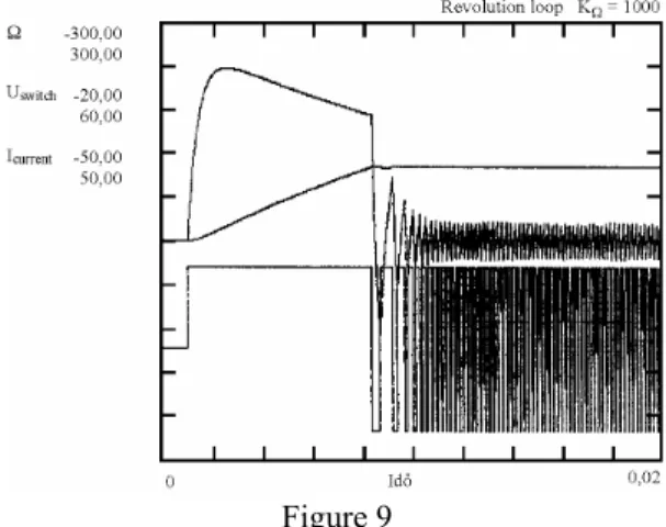
Under the same conditions in what has gone before KΩ=1000. Non-damping vibrations set in. By increasing the proportional coefficient of amplification the accuracy of regulation can be increased, but problems of stability can arise.
Figure 9 Effect of drive inertia. Reduction on motor-axis.
Figure 10
at t=50 ms; Ube=7.209 V; Ia=6.092 A; Ω=99.994 r/s; Θ=3Θrotor On the basis of capacity:
Mr ⋅nm =Mload ⋅nload⋅1
η (14)
η - transmission efficiency
M M n
n M
r load load
motor
= ⋅
⋅ = load⋅a
⋅
η η
1 (15)
Kinetic energy:
1 2
1 2
Θload⋅Ω2load = Θ Ωr ⋅ 2m⋅ η (16)
Θr Θlo a d
= ⋅ a
⋅ 1
η 2 (17)
In accordance with the relationship follows that in the case of reducers inertia of the driven arm has less influence. If the reduced inertia can be compared with the rotor inertia as it seen in Fig 6, regulation slows down (T increases) and the current load of the armature considerably increases.
Building up the regulating circle for the position.
3 The Position Control
Feedback of the proportional regulating loop for the position is performed by potentiometer.
Figure 11
Kα proportional coefficient of amplification influences accuracy and stability of regulation. (Fig. 7, 8, 9)
As it seen from the diagrams that the proportional coefficient of amplification is sensitive to the scale of amplitude in the base signal. The inertia of the driven arm consideratly impackt on the quality of control, too.
The Whole circuit design Was concluded by the solution of the position control.
Funktion between αfault (s) and Ωbasis (s):
K⋅sTi +
1 1 1
s T a s T
d d
+ ⋅ + ⋅ ⋅
(18)
where Ti integration
Td differential time constant K amplification factor
at a=1 or Td=0 PI regulation can be achieved
Figure 12
Mt =0 influence of the proportional coefficient of amplification Kα=300 aperiodic Kα=500 aperiodic with swing-off Kα=1000 periodic, with damped vibration.
Figure 13
Mt=0 at t=100 ms; α=19.899; Ube=-0.009 V; Ia=-0.386 A
Kα proportional factor of amplification should be the function of the basic signal amplitude. Kα=300 set in to the 40° junp at 90° jump results swing-off, by decreasing of it the accuracy depreciates.
Θ = Θrotor aperiodic swing-off free set in of the rotor.
Θ = 3Θ rotor aperiodic set in of the rotor with swing-off
at t=50 ms; Ube=0.028V; α=40.008°; Ia=0.095 A; Ω = -0.043 r/s
Figure 14
If the inertia of the arm can be compared with the inertia of the rotor - so in that case it has a great influence on the position regulating circle, too. The quality of range changes under the same contitions and so does the range time.
Figure 15
Parameters: K=100; Td=10-3; a=0.05; Mt=0; t=150 ms; Ia=-0.006 A; Ube = 0.0028V; α = 19.998°; Ω = 0.0018 r/s
Θ = Θrotor her initial run-up takes place faster
Θ = 3Θ rotor, then run-up is slower but the set-in (has the) same quality.
Θ = 3Θrotor at t=50 ms; Ube=-0.025V; α=39.976°; Ω=0.068 r/s
Figure 16
Fig. 16 repetation of simulations Fig 14. with PD control
Figure 17
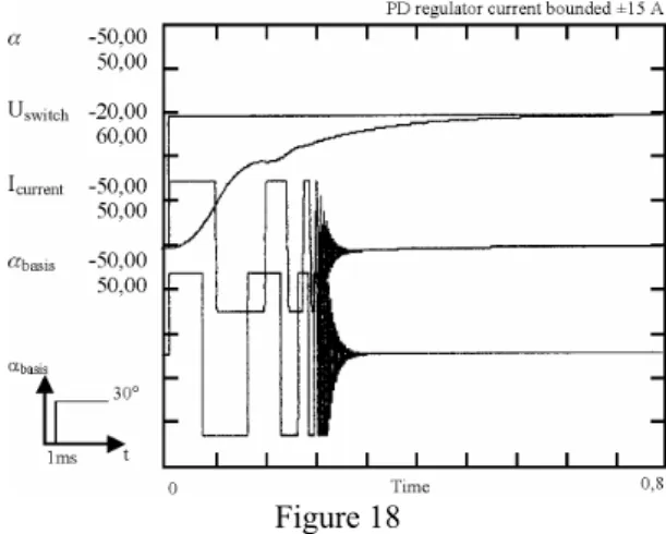
As it seen that in most part of reset time great amount of current falls to the armature. At starting without current limit, cca 39 A peak current appears.
Amplification factor of PID member is: K=200
Mt=0 Amplification factor as the PID member should be decreased by K=80 for stabilitys sake. Setting time increases signifcantly.
In the case of real load control into the positions station can be very quick, so in every starting much current load to be reckoned wicht.
The motor in unable to bear in a long run. Current belonging to its nominal moment is 6,1 A but at starting it is 5-6 times more.
Figure 18 Conclusions
In accordance with these principles the presentation is rich in illustrations selected from the ample set of particular investigations. Though the limited size of this paper does not make it possible to give the full description of the verification of
the models applied, it is worthy of note, that via completing wide-spread series of simulations and measurements the appropriate models have been verified.
The main aim of the here published development was to bring about an open motion control system for a robot used for educational purposes.
References
[1] I. J. Rudas, L. Horváth: Fault Detection in Industrial Robots Using a Learning Control Based Approach. Proc. of the 32nd SICE Annual Conference. Kanazawa, Japan, 1993.
[2] Dr. Attila Bencsik-György Suszter: Investigation of Robot Arm Ridigity Mechatronics Vol. 3. No. 2. pp. 185-203 1993.
[3] A. Bencsik, I. J. Rudas: Simulation Tool for Interactive Design of Force Reflecting Master Arms. Bulletins for Applied Mathematics 947/94. The 25th Year’s Jubilee Meeting in London, United Kingdom. pp. 99-105.
[4] Givon C. K. Yan, Clarence W.de Silva and George X. Wang Simulation and experiments on Intelligent control of a Wooddryng Kiln. IFAC Symposion on Artifical Intelligence in Real Time Control (AIRTC-2000) Budapest, Hungary, Preprints pp.75-79.
[5] Ales Hace, Karel Jezernik :Robust Position Tracking Control for Direct Drive Robot Proceedings of the International Conference on Itelligent Engineering Systems (INES 2000), Portoroz, Slovenija, pp. 121-124.