Let your maps be fuzzy! — Class probabilities and floristic gradients as alternatives to crisp mapping for remote sensing of vegetation

(1)

Let your maps be fuzzy! — Class probabilities and floristic gradients as alternatives to crisp mapping for remote sensing of vegetation

Hannes Feilhauer^1,2,3 , Andras Zlinszky⁴ , Adam Kania⁵, Giles M. Foody⁶ , Daniel Doktor^2,7, Angela Lausch^8,9 & Sebastian Schmidtlein¹⁰

1University of Leipzig, Talstr. 35, 04103 Leipzig, Germany

2Remote Sensing Centre for Earth System Research, Leipzig University & Helmholtz Centre for Environmental Research–UFZ, Talstr. 35, 04103 Leipzig, Germany

3Freie Universit€at Berlin, Institute of Geographical Sciences, Malteserstr. 74-100, 12249 Berlin, Germany

4Centre for Ecological Research, Balaton Limnological Institute, Klebelsberg Kunout 3, 8237 Tihany, Hungary

5Definity, Wrocław, Poland

6School of Geography, University of Nottingham, Nottingham, England

7Department Remote Sensing, Helmholtz Centre for Environmental Research–UFZ, Leipzig, Germany

8Department Computational Landscape Ecology, Helmholtz Centre for Environmental Research–UFZ, Leipzig, Germany

9Geography, Humboldt Universit€at Berlin, Unter den Linden 6, 10099 Berlin, Germany

10Karlsruher Institut f€ur Technologie (KIT), Institut f€ur Geographie und Geo€okologie, Karlsruhe, Germany

Keywords

ecotone, floristic gradient, fuzzy

classification, gradual transition, ordination, vegetation mapping

Correspondence

Hannes Feilhauer, University of Leipzig, Talstr.

35, 04103 Leipzig, Germany. Tel:+49-341- 235482335; Fax:+49-341-9732809; E-mail:

hannes.feilhauer@uni-leipzig.de Editor: Kate He

Associate Editor: Mat Disney

Received: 19 July 2020; Revised: 2 October 2020; Accepted: 2 November 2020 doi: 10.1002/rse2.188

Remote Sensing in Ecology and Conservation2021;7(2):292–305

Abstract

Mapping vegetation as hard classes based on remote sensing data is a frequently applied approach, even though this crisp, categorical representation is not in line with nature’s fuzziness. Gradual transitions in plant species composition in ecotones and faint compositional differences across different patches are thus poorly described in the resulting maps. Several concepts promise to provide better vegetation maps. These include (1) fuzzy classification (a.k.a. soft classification) that takes the probability of an image pixel’s class membership into account and (2) gradient mapping based on ordination, which describes plant species composition as a floristic continuum and avoids a categorical description of vegetation patterns. A systematic and comprehensive comparison of these approaches is missing to date. This paper hence gives an overview of the state of the art in fuzzy classification and gradient mapping and compares the approaches in a case study. The advantages and disadvantages of the approaches are discussed and their performance is compared to hard classification (a.k.a.

crisp or boolean classification). Gradient mapping best conserves the information in the original data and does not require ana priori categorization. Fuzzy classification comes close in terms of information loss and likewise preserves the continuous nature of vegetation, however, still relying ona priori classification. The need for a priori classification may be a disadvantage or, in other cases, an advantage because it allows using categorical input data instead of the detailed vegetation records required for ordination. Both approaches support spatially explicit accuracy analyses, which further improves the usefulness of the output maps. Gradient mapping and fuzzy classification offer various advantages over hard classification, can always be transformed into a crisp map and are generally applicable to various data structures. We thus recommend the use of these approaches over hard classification for applications in ecological research.

(2)

Introduction

Remote-sensing-based vegetation mapping has boosted both ecological science and conservation practice. The generated maps aim to provide detailed information on the distribution of patterns in plant species composition, similar to maps produced through field surveys. These maps thus contain more information on vegetation than conventional remotely sensed maps that often consider coarse land cover classes only. Frequently, the workflow of respective mapping approaches requires a system of pre-defined, discrete vegetation classes and assigns each image pixel unambiguously to one (and only one) of these classes. The resulting map displays hard, crisp boundaries delineating categorical mapped units with an assumed species composition. This approach generates maps that are easy to read for human beings since they meet the human tendency to think in categories. On the other hand, this categorization of vegetation with gradual transitions in plant species composition is not always in line with reality (as already pointed out by Gleason, 1926); hard boundaries are sometimes found in reality, but ecotones or soft transitions are also widespread (Fig- ure 1). Even if hard boundaries prevail, like in some cul- tural landscapes, patches of the same categorical unit still differ slightly in their species composition. It is important to note that while the concept of ecotones describes a transition in geographical space, transitions in species composition in the feature space are likewise inappropri- ately dissected by hard classifications. By forcefully apply- ing data structures designed for discriminating objects of homogeneous (bio-)physical characteristics to land surface elements exhibiting a mixture of different objects, hard classification causes problems regarding class definitions, mapping accuracy, and applicability for many real-world vegetation types: crisp categorization systems often do not describe fuzzy vegetation patterns well and do not serve the application needs sufficiently (de Klerk, Burgess, &

Visser, 2018). The attempt to describe these patterns in a more realistic manner is referred to as fuzzy mapping.

Fuzzy mapping in a strict sense is based on fuzzy set theory (Zadeh, 1965), an alternative to the commonly used classical set theory in hard classification. According to classical set theory, the definition of a set (group, class, category) is adequate when it allows to decide unambiguously whether an observation is an element of the set or not. Hard classification is therefore typically designed to be non-overlapping. In contrast, the fuzzy set theory allows partial membership of an entity in one or more sets at the same time. The level of membership is described by a scalar value between zero and one. Each entity has a class membership vector with as many elements as classes defined, each element representing the

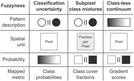
level of membership in that specific class. Typically, the class membership vector is expected to add up to 1. In vegetation mapping, main sources of fuzziness are frequently considered in classification (Figure 2): (1) the uncertainty of class membership per mapping unit,

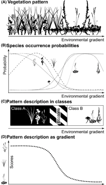
Figure 1. (a) & (b) Species distributions along an environmental gradient. Species occurrence probabilities are changing according to the ecological demands of the species and processes in the community. This forms spatial patterns in plant composition determined by the prevailing environmental conditions at the respective sites. Note that this continuum does not need to be spatially continuous; it can also be found in scattered patches. (c) Description of patterns in species composition as discrete plant assemblages. Gradual transitions are described as ecotones, where one class is gradually replaced by another. (d) Description of patterns in species composition as a floristic gradient. The gradient scores change gradually with changing species composition. Both concepts can be used to map vegetation with remote sensing.

(3)

thereby assuming that the mapping unit belongs with a certain probability to one or more classes (Rocchini, 2010) and (2) the description of a fine-scale, heterogeneous mixture of classes within a mapping unit as cover fractions (Foody, 2002). A discussion of these approaches for mapping discrete classes is provided by, for example, Wang (1990) and Foody (1996). An alternate approach (3) is to map the vegetation patterns without classification, describing gradual changes in the species composition as continuum (Schmidtlein & Sassin, 2004; Trodd, 1996).

These three approaches thus link to two alternate concepts in the field of vegetation science: Clements’ (Cle- ments, 1916, Figure 1c) and similar approaches like the Braun-Blanquet phytosociological approach describe typical plant communities or vegetation types through char- acteristic species occurrences along environmental gradients. Each resulting unit is defined by a distinct set of species, resulting in a hard classification. Ecotones are addressed through the definition of transition classes. In contrast, Gleason’s continuum concept (Gleason, 1926) considers overlapping the ecological demands of the individual species and challenges the idea of regularly co-occurring species. The sum of species-specific occurrence probabilities along environmental gradients translates into gradual transitions in plant species composition (Fig- ure 1d). These gradients can be extracted from vegetation data using ordination techniques that enable a class-less (i.e., continuous) pattern description.

Both concepts can provide a fuzzy and more realistic description of the actual patterns in species composition (Figure 2) compared to hard classification. The whole

process of remote-sensing-based hard vegetation classification is based on finding ‘pure’ pixels for training and evaluation, therefore requiring unambiguous information.

When this is applied to vegetation data involving uncertain class memberships, problems arise. Fuzzy mapping approaches hence further promise an increase in classification performance and accuracy (Shanmugam et al., 2006).

With the onset of quantity disagreement and allocation disagreement (Pontius, 2002), the accuracy assessment of crisp maps may have reached its technical limit: Scalar quantities accurately define the two kinds of classification error, but are still based on the assumption that the validation data are a perfect representation of the map prop- erties and that classification accuracy is homogeneous at least for every class throughout the mapped area. Fuzzy classification likewise enables confusion matrix-based indices (Binaghi, Brivio, Ghezzi, & Rampini, 1999; Kumar

& Dadhwal, 2010; Silvan-Cardenas & Wang, 2008) but also a spatially explicit accuracy assessment (Foody, Campbell, Trodd & Wood, 1992; Zlinszky & Kania, 2016), which is out of the reach of hard boundary data.

Despite the various alternatives, recent applications of remote sensing in vegetation mapping are still dominated by hard classification and thus possibly affected by various drawbacks. We observe that non-crisp vegetation classification has not become mainstream over the last decades for several reasons. These include the lack of standard procedures especially for accuracy assessment, the scarcity of appropriate reference data, the need for computing power and difficulties with the visualization of the results. Many of these limitations have recently been

Figure 2. Ways to consider the fuzziness of vegetation in remote-sensing derived maps. The fuzziness can be expressed by mapping the uncertainty of class membership, by mapping cover fractions of classes within a pixel based on spectral similarities to reference data (note that the grid indicates fractions, not a finer spatial resolution), or by describing the species composition as class-less continuous metric.

(4)

overcome: new standards of accuracy assessment for fuzzy maps have been suggested (Binaghi et al., 1999), high- throughput biodiversity quantification methods allow rapid collection of reference samples without the need for a priori classification (Bush et al., 2017), visualization methods have been developed and computing capacity is rapidly increasing. Additionally, soft classification allows calculating pixel uncertainty in a spatially explicit way (Khatami, Mountrakis, & Stehmann, 2017) adding information beyond the spatially unresolved accuracy indices classically used for Boolean categorizations. In the opera- tional case, a detailed understanding of the error distribution in space leads to better reference sampling strategies and more critical use of the output information (Zlinszky

& Kania, 2016).

It is thus from our point of view not clear why hard classification should be further preferred over any approach that allows to map the fuzziness in species composition illustrated in Figure 2. Is it traditionalism, the compulsion to discrete and simplified output from the users, or the sheer variety of available approaches, each with their own advantages and disadvantages? These range from ensemble or probabilistic classifiers applied to crisp data structures through generating a fuzzy output map based on a set of samples that are pure class instances, to using fuzzy data structures from the start to the end of the workflow (Foody, 1999). The ultimate level of non- crisp vegetation mapping is to eliminate categories completely and to map species occurrence data directly via floristic gradients, as in ordination. Deciding which one to use is a non-trivial task, which, as we suspect, is often evaded by the shortcut of defaulting to classical hard- boundary mapping. We hence aim in the present paper to describe and compare non-crisp approaches within remote sensing-based vegetation mapping. We use a comparative study to illustrate the principles and differences, including opportunities for accuracy assessment, between the two main fuzzy alternatives, using hard classification as a benchmark. Since each general approach has its advantages, the main intention of this comparison is to provide a guideline when and how to use fuzzy approaches to avoid hard classification.

Materials and Methods

Study area and data

The comparative case study was conducted in an extensively used mosaic of raised bogs, transition mires, poor fens and grasslands in the Bavarian alpine foothills in Southern Germany (47.74° N, 11.08° E). The study area and its vegetation are described in detail in Feilhauer et al. (2014) and Feilhauer, Doktor, Schmidtlein and

Skidmore (2016). In this area, 100 randomly arranged vegetation plots covering 4 m² each were sampled. In each plot, cover fractions of all occurring vascular plant species as well as the cover fractions ofSphagnummosses and other bryophytes were estimated. The resulting plot by species matrix was used to characterize the plots’ species composition. This matrix was subjected to a cluster analysis for classification and ordination for gradient mapping, in both cases aiming to extract the predominant patterns in species composition.

Hyperspectral imagery of the study area with a ground resolution of 2 m x 2 m was acquired on 16 Jul 2013 with the airborne AISA Dual sensor in four overlapping flight lines. The data cover the spectral range from 407 nm to 2499 nm in 366 spectral bands. Reflectance spectra of the plots were extracted from the radiometri- cally, geometrically and atmospherically corrected raw imagery using the GPS coordinates of the plot centers.

For more information on the image data acquisition and processing, please refer to Feilhauer et al. (2014, 2016).

Gradient and cluster analysis of the vegetation data

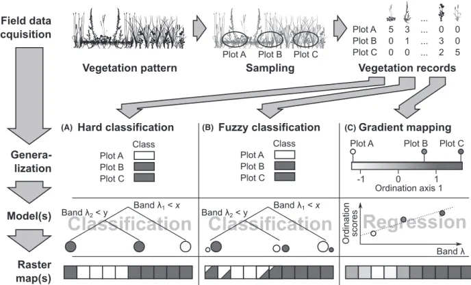
Figure 3 shows the schematic workflows for hard and fuzzy classification as well as for gradient mapping. To describe the gradual transitions in species composition as floristic gradients, the vegetation plot data were subjected to an ordination, specifically isometric feature mapping (Isomap, Tenenbaum et al., 2000). We chose this particular technique because it compared favorably to other ordination techniques in a previous study (Feilhauer et al., 2011) and shares a common methodological basis with the cluster analysis technique described below. Iso- map, as other ordination techniques, determines the mutual inter-plot Bray-Curtis dissimilarities regarding species composition and projects these relations to a low- dimensional floristic feature space. Plots that show a similar species composition are located nearby in the resulting multidimensional ordination space; plots with a very dissimilar species composition are located far from each other. The axes of the ordination space have a hierarchi- cally decreasing information load and correspond to floristic gradients that are treated as measures of gradual changes in species composition. Numerical plot positions on these gradients (i.e., axis scores) are thus an indicator of plant species composition and can be interpreted accordingly.

For hard and fuzzy classification, the data were subjected to a cluster analysis (isopam; Schmidtlein, Tichy, Feilhauer, & Faude, 2010). The isopam approach was chosen because it is based on a partitioning of isomap ordination spaces and offers an advantage over other

(5)

clustering techniques: The clusters are identified in a data-driven way as groups of plots with a similar species composition that is characterized by a set of indicative species. The list of species is provided as part of the output.

Hard and fuzzy classification of the imagery For fuzzy classification, we chose the mapping of class membership probabilities over sub-pixel class cover fractions. Many classification approaches commonly used in the field of remote sensing such as, for example, maximum likelihood or random forest (RF, Breiman, 2001) are actually based on calculating class probabilities and discretize the membership in the last step, therefore in these cases, a fuzzy output is a by-product at no extra processing cost. Mapping cover fraction requires more customized approaches such as, for example, spectral unmixing. For this reason, we considered probability- based fuzzy mapping the more straight-forward approach.

Here, we used RF classification to map the plot-based isopam clusters. Based on the pixel’s spectral characteristics, RF predicts the most likely vegetation class as well as the class probability or certainty of assignment, making RF suitable for both hard and fuzzy classification. While a

validation of the models against an independent dataset in general considered more reliable, we opted for the use of an out-of-bag error assessment due to the limited number of vegetation plots. We applied the RF model in both prediction modes on the image data. This returned on the one hand a pixel-wise prediction of the spatial isopam cluster distribution as a hard classification result and on the other hand a separate map for each cluster displaying the pixels’ membership probabilities. The latter was used as a fuzzy classification result in our comparison. Additionally, for visualization purposes, a ‘blended’

map was produced by assigning specific colors to each of the isopam classes and generating a color mixture from a weighted probability average of the individual class colors.

In both predictions, pixels covering forest, agricultural areas and artificial surfaces were masked using a pre-existing land-cover map.

Gradient mapping

Following Schmidtlein et al. (2007), the ordination axes scores of the plots were regressed against the reflectance spectra using Partial Least Squares regression models (Wold, Sj€ostr€om, & Eriksson, 2001). A separate model was built for each axis. Model fits were assessed with ten-

(A) (B) (C)

Figure 3. Workflows for (A) hard classification, (B) fuzzy classification and (C) gradient mapping. The three concepts differ in the description of the vegetation patterns (classes vs. gradients), in the modeling approach and in the map representation of the patterns.

(6)

fold cross-validation. Again, a validation against independent data may be more desirable, but was not used due to the limited number of vegetation plots. Subsequently, the models were applied to the image data to predict each pixel’s position on the ordination axes. The resulting maps were merged into a color composite. Likewise, all areas that were not represented by the vegetation sample were masked.

As a graphical legend for this gradient map, the Isomap ordination space was translated into RGB color gradients.

The rescaling factor of the numerical axis scores to RGB triplets corresponded to the color stretch of the composite map. The position of a plot and likewise the predicted pixel position on the gradients is thus expressed in a unique color value. Plots and pixels with a similar color hence feature a similar species composition.

Assessing the information loss and mapping uncertainty

For an objective comparison of the three methods, we assessed for each approach the loss of information from the original vegetation data to the final map. For this purpose, we extracted the predicted hard class membership, fuzzy probabilities and gradient scores for each plot from the maps. The categorical class membership predictions were converted into dummy variables, that is, a four-column matrix with one column per class and binary values indicating the predicted class membership of each vegetation plot. We then calculated the Euclidean distances between the plots from these prediction results and performed a correlation analysis against the Bray-Curtis distances of the plots calculated for the original vegetation data. The squared Pearson R of these correlations was used as a measure of the original information that was preserved through generalization and modeling. A R²=0 indicates a full information loss, a R²=1 indicates full preservation of the original variation. Obviously, the results of this comparison are highly dependent on input data and model performance and cannot be taken as being globally valid. However, they allowed for a better understanding of how much detail is preserved in the final maps.

Additionally, we aimed to quantify the mapping accuracy by comparing the similarity of the predicted species composition to the species composition observed in the field. For hard classification, the standard way to quantify this is through a confusion matrix, which summarizes the correctly identified and misclassified reference pixels for each class. This approach does not deal with transitions between classes or uncertainty of categorization. For evaluating the accuracy of the fuzzy classification approach, we thus used the ‘fuzzy confusion matrix’ (Zlinszky &

Kania, 2016). This matrix takes the output of the individual base clasifiers (here decision trees in the random forest) into consideration and quantifies for each reference pixel the percentage of base classifiers that voted for a particular class. The resulting matrix produces class-wise or overall accuracy metrics that are inherently lower than or equal to their equivalents in the hard matrix. This is because the fuzzy confusion matrix takes the uncertainties of assigning each pixel to a class into account: more certain assignments (whether right or wrong) produce higher numbers, less certain assignments give lower numbers in each cell of the confusion matrix. If all base classifiers for all the pixels in a confusion matrix cell output the same class, the value in that cell will be identical to the same cell value of a hard confusion matrix. If this is not the case, the fuzzy confusion metrics are lower. However, the fuzzy confusion matrix provides a more sensitive way of judging the quality of a classification output (Zlinszky &

Kania, 2016).

Further, we aimed to visualize the uncertainty of the pixel-wise predictions. For hard classification, we mapped for each pixel the F1-score related to the predicted class membership. The F1-score or F measure (Hand, 2012) provides a class-wise summary of the precision (i.e., the proportion of true positives in all data points assigned to a class) and recall (i.e., the percentage of true positives in the correct predictions) of the predicted class memberships. A high F1-score indicates that the class prediction is unambiguous. However, besides the issue that this measure is not spatially explicit but only related to the predicted class, a second problem emerges: if two classes achieve similar probabilities, the prediction is likewise ambiguous, even for high probability values. For fuzzy classifications, several possible metrics of pixel-wise certainty have been proposed based on the class membership probabilities, addressing the question ‘did the final class get only a marginal majority of the votes or was the decision unambiguous’? Here, we used the probability-surplus index (Zlinszky & Kania, 2016) for this purpose. This index quantifies in a spatially explicit way for each predicted pixel the difference in probability between the most likely and the second-most likely class, illustrating the unambiguity of the prediction. For the gradient map, we used an approach described in Feilhauer, Faude, and Schmidtlein (2011) based on the ideas of Janet Ohmann (Ohmann & Gregory, 2002; Ohmann, Gregory, Hender- son, & Roberts, 2011). For each pixel, we calculated the minimum distance to the nearest-neighbor plot in the gradient space. This distance indicates whether a plot with a similar position in the gradient space and hence a similar species composition has been sampled in the field. A relatively large mapped gradient-space distance indicates that the respective pixel is rather dissimilar to all field

(7)

plots. The prediction for this pixel has thus a rather high uncertainty. Likewise, a pixel that is spectrally dissimilar to all field observations will have a predicted position on one of the far ends of the gradients and thus feature a large minimum distance in the index map.

Results

Clustering and ordination of the vegetation data

Isopam cluster analysis resulted in a hierarchical classification of the plots. At the first, coarsest level, fen and grassland plots were separated from plots in transition mires and raised bogs. At the second level, both clusters were further divided, resulting in a total of four classes. Cluster 1.1 includes 30 plots from calcareous, nutrient-poor fens and Molinia grasslands, cluster 1.2 consists of 31 plots from extensively used, calcareous and fresh meadows, cluster 2.1 contains 15 plots from transition mires and cluster 2.2 includes 24 plots from the raised bogs.

For the Isomap ordination, we opted for a two-dimensional solution resulting from k =15 that explained 68%

of the original variation. The first axis describes the gradual transition in species composition from calcareous grasslands and poor fens via transition mires to the acidic raised bogs. The second axis quantifies compositional changes from calcareous sites into poor fens and Molinia grasslands.

Model fits

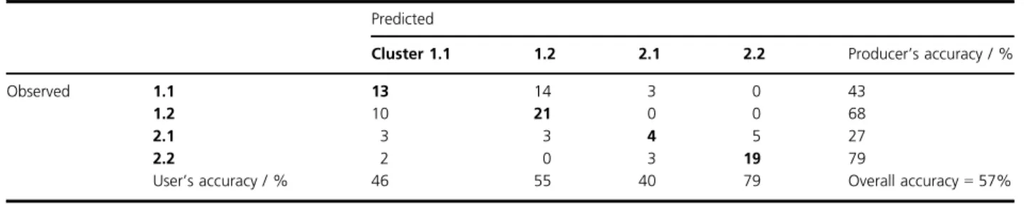
The RF classification model gained an overall accuracy of 57% as quantified by the out-of-bag error. Errors are mostly due to confusion between the grassland and poor fen clusters 1.1 and 1.2. In particular, the raised bog cluster 2.2 was modeled with a rather high user’s and producer’s accuracy of 79%. Table 1 shows the confusion matrix and the resulting user’s and producer’s accuracies. Considering the model fit at the coarser level of the cluster analysis, separating only cluster 1 and cluster 2, the overall accuracy increases to 89%. Like- wise, when clusters 1.1 and 1.2 are merged, the resulting overall accuracy is still 81%. Based on the fuzzy confusion matrix, the overall accuracy for the four classes was 52% (Table 2). The decrease in accuracy compared to the Boolean confusion matrix is due to the substantial probabilities assigned to incorrect classes: in most cases, the prediction of even the correct class had probabilities well below 100%.

The cross-validated PLS regression models for Isomap gradient 1 resulted in a R²cal =0.86 and R² val=0.79 as well as RMSEcal=0.28 and RMSEval=0.34. The model for

gradient 2 had a weaker fit and resulted in R²cal =0.58 and R²val=0.471 with RMSEcal=0.24 and RMSEval=0.27.

Both models were based on six latent vectors that sum- marize the spectral information.

Maps of plant species composition

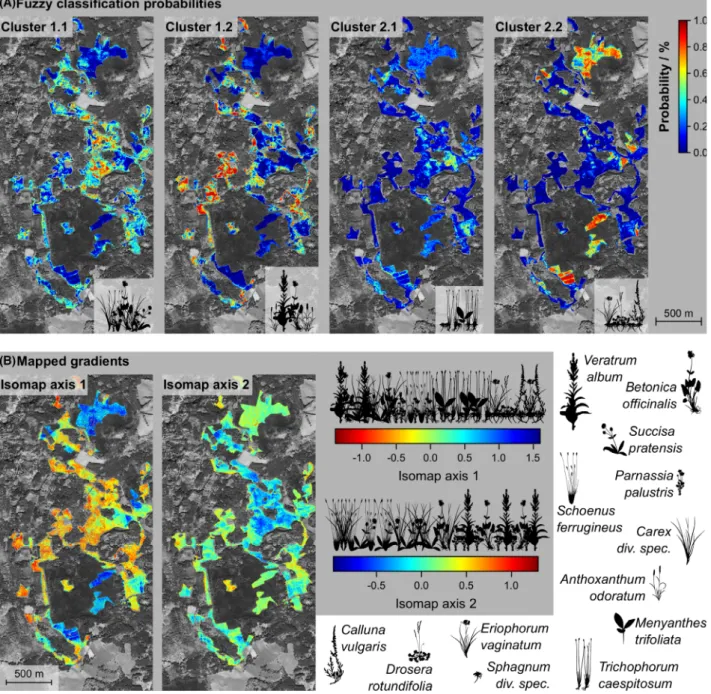
The resulting maps of fuzzy class probabilities and ordination scores are displayed in Figure 4. Fuzzy classification provides a separate map for each cluster (Figure 4a), illustrating the pixel-wise probability of class memberships. Gradual transitions in plant species composition emerge as gradual probability changes, showing the spatial transition from one class to another. The gradient map (Figure 4b) shows for each pixel the predicted position on the Isomap axes. In these maps, the pixel values correspond to the numerical gradient scores that indicate the respective species composition along the respective gradient.

The blended map color composites of the individual maps are displayed in Figure 5. This figure also presents the hard classification map (Figure 5a). In the blended fuzzy map (Figure 5b), the mixtures of the four primary color hues indicate the predicted transitions between the four clusters. The RGB gradient map (Figure 5c) illus- trates for each pixel the color-coded position on the Iso- map gradients. This allows to estimate the pixel’s predicted species composition.

Information loss and maps of uncertainty The Pearson correlations between dissimilarities of the original vegetation data and modeled and predicted Iso- map axis scores resulted in R²=0.42, indicating that 42%

of the original information content is preserved in the gradient map. The fuzzy and hard classifications resulted in R²=0.40 and R²=0.31, respectively.

Mapped uncertainties for the classification approaches are shown in Figure 6a and b, the uncertainties for gradient mapping in Figure 6c. Map 6c indicates that only small parts of the mapped area are not represented by the field sampling.

Discussion

Ability to represent fuzzy patterns

Hard classification further preserved a considerably lower percentage of information as compared to fuzzy classification and gradient analysis, which showed a similar ability to describe the variation in the plot vegetation data. The order of magnitude of differences in information loss depends on many factors such as the data used, the set of

(8)

classes defined and their ability to describe differences in vegetation, and methodological details. We believe, however, that the pronounced differences between fuzzy and hard classification, being based on the same data generalization and the same model, can be reliably taken as typical for the information loss that results from hard classification.

As expected, both fuzzy classification and gradient mapping are suitable to depict fuzzy vegetation patterns.

The map representations in Figure 5b and c meets the distribution observed in the field. Hard classification is unable to describe gradual transitions and introduces artificial boundaries that are not in line with our field observations. The only viable solution to map gradual transitions with hard classification is the definition of transitional classes. However, this workaround requires a large number of transitional classes for an accurate description and thus interferes with the ease of interpreta- tion, which is otherwise the main advantage of hard classification.

Hard classification as well as fuzzy classification of the image data have in common thata prioriclass definitions need to be taken. Here we used isopam cluster analysis, but numerous alternatives including the global classification approaches proposed in phytosociology or habitat classification schemes exist. In vegetation science, classification per seis not always seen as appropriate to describe vegetation patterns. Considering this uncertainty, the need fora priori classification may be a drawback in comparison to gradient mapping. Nevertheless, fuzzy classification is still

versatile in mapping gradual transitions (de Klerk et al., 2018). The class distribution patterns in Figures 4a and 5b illustrate this ability. We frequently observe transitions from a high to a low probability of one class and corre- sponding, inverse patterns for the other classes that allow to estimate the fuzzy transitions. A drawback of fuzzy classification is the presentation of the patterns across multiple maps. Three of these maps can be combined to an RGB composite, assigning one color component to the map of a class. Alternatively, as done here, a color can be assigned to each class and blended to represent the level of membership for each pixel. For the four maps resulting from our case study, this presentation is still manageable. However, if a larger number of vegetation classes is considered, the colors representing the individual classes may not be distinguish- able.

Gradient mapping is highly capable of displaying fuzzy transitions. In our case study, all transitions in plant species composition become apparent at the first glance.

Since the approach treats every vegetation stand as an individual mixture of species—in line with Gleason’s individualistic concept of the plant assemblage—its abili- ties to deal with fuzzy patterns may be considered supe- rior. Likewise, the resulting maps can be displayed individually or as a color composite of up to three gradient maps. This is almost always sufficient as ordination results only in rare cases in more than three meaningful axes. Statistically speaking, the output is provided as an interval-scaled variable, which supports further analyses and modeling.

Table 1. Confusion matrix of the random forest classification model and class-specific user’s and producer’s accuracies.

Predicted

Cluster 1.1 1.2 2.1 2.2 Producer’s accuracy / %

Observed 1.1 13 14 3 0 43

1.2 10 21 0 0 68

2.1 3 3 4 5 27

2.2 2 0 3 19 79

User’s accuracy / % 46 55 40 79 Overall accuracy=57%

Table 2. Fuzzy confusion matrix of the random forest classification model and user’s and producer’s accuracies.

Predicted

Cluster 1.1 1.2 2.1 2.2 Producer’s accuracy / %

Observed 1.1 13.41 9.73 4.90 1.96 45

1.2 10.35 18.77 1.28 0.60 61

2.1 4.24 1.71 4.22 4.83 28

2.2 2.15 0.72 5.76 15.37 64

User’s accuracy / % 44 61 26 68 Overall accuracy=52%

(9)

Like local classification schemes, ordination axes are not comparable across study sites unless extra measures are taken. Such measures include a projection of new data points based on primary ordination space loadings. How- ever, the use of a ‘global’ gradient as equivalent to a pre- defined classification key is practically hardly feasible.

Also, for vegetation data with very high variation, fine differences are difficult to map (Unberath et al., 2019).

Common regression techniques, including machine

learning, frequently fail to model and map the resulting gradients in such cases. A general drawback of gradient maps is that area statistics are not available without further classification of the continuous map. Gradients are also not in line with the human tendency to think in categories. In consequence, potential users often find the gradient concept less intuitive compared to a classification and need some time to adjust themselves to the gradient map and legend.

Figure 4. Fuzzy representations of the vegetation patterns resulting from (A) fuzzy classification and (B) gradient mapping. The four panels in (A) illustrate the isopam cluster membership probabilities. The two gradient maps in (B) display the predicted position of each pixel on the Isomap axes 1 and 2 as indicator of plant species composition.

(10)

Figure 5. Final vegetation maps for the northern part of the study area resulting from the three mapping approaches. (A) Class membership of each pixel as predicted by hard classification. (B) Blended probability map for the four isopam clusters resulting from fuzzy classification. (C) Gradient map resulting from Isomap ordination and regression modeling. Areas not represented by the vegetation sampling such as forests and intensively used grasslands are masked.

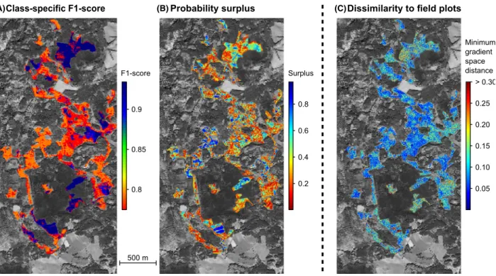
(A) (B) (C)

Figure 6. Maps of mapping uncertainty. (A) F1 score per predicted class for hard classification. (B) Probability surplus index per pixel as a measure of ambiguity of the prediction in fuzzy classification. (C) Minimum Euclidean distance per mapped pixel to the nearest neighbor plot in the ordination space indicating how well the predicted species composition is represented by the field sampling.

(11)

Hybrid approaches that take advantage of both worlds exist. Several studies used gradient analyses to generalize the vegetation data of their study area and mapped the gradient scores with nearest neighbor estimation to avoid extrapolation (Ohmann & Gregory, 2002; Ohmann et al., 2011; Thessler, Ruokolainen, Tuomisto, & Tomppo, 2005), treating each plot as an individual class. Still, the result is metrically scaled even though not presented in continuous values. These hybrid approaches enable area statistics in addition to the advantages of gradient mapping. They are, however, more affected than conventional gradient mapping by an uneven representation of mixed plant assemblages present in the study area.

Spatially explicit accuracy assessment

The accuracies obtained in our case study are fair but not exceptionally high for all three approaches. For classification, the outputs show that some clusters were more difficult to map than others: cluster 2.1 (transition mires) had the lowest producer’s and user’s accuracies in the hard confusion matrix. The even lower values in the fuzzy confusion matrix show that the identification of this class was often with higher ambiguity compared to the other classes. However, it is important to note that the accuracy metrics can not be directly compared. Fuzzy classification is not 5% more inaccurate than hard classification: Since both classification results are retrieved from the same model (but taking into consideration different outputs), the overall accuracy calculated for the class memberships with the highest probability is likewise the same.

Meanwhile, hard boundary maps and their accuracy metrics are based on the rarely fulfilled assumption that classification accuracy is a class-specific attribute, that is that it is homogeneous across the mapped area. In typical workflows, this may refine the classification by, for example, increasing the sample for the classes showing the worst performance (Foody et al., 1992), or balancing over- and underestimation by tweaking the algorithm.

However, this does not allow to evaluatewhereclasses are confused. For low accuracies, model development often has to resort to trial and error.

For fuzzy classification, the probability surplus map or similar approaches suggested by Oldeland, Dorigo, Lieck- feld, Lucieer and J€urgens (2010) and Duff, Bell and York (2014) are helpful in assessing uncertain areas independent from the respective pixel’s class membership. This means that even in the case where most pixels of a class are accurately mapped, an uncertain location can be identified. From the user perspective, such a spatially explicit accuracy assessment allows to be cautious wherever certainty is inadequate, or to use alternatives for making decisions in that specific location. Additionally, in an

active learning setup, sampling can be iterated until the desired accuracy is reached.

Finally, for ordination, the map of gradient distance to the most similar sampling plots aids the refining of sampling to cover the gradient space. It also provides information on species composition: species that were not present in the plots will most likely occur in the areas where the gradient distance is high, and any management activities that are based on the map should be applied with caution in these locations due to high local uncertainty.

Data requirements

Fuzzy mapping approaches differ considerably in their requirements regarding the vegetation input data. Gradi- ent mapping is only feasible if a plot-by-species matrix listing the species occurrences per plot is available. This matrix is the basis for ordination and cannot be replaced by any other means. To generate a gradient map, field- work has to include the costly and time-consuming sampling of full vegetation records, unless plot data are available from databases. Various scales can be used to record the plant species composition of the plots, including measured or estimated cover fractions, dominance and abundance scales. Gradient analysis is able to handle all of these data; however, from a remote sensing point of view, an estimation in quantitative cover fractions should in theory be preferred over presence–absence data because species with high cover in the upper canopy contribute predominantly to the spectral signal.

Fuzzy classification approaches are more flexible in terms of data requirements since they can be simply built upon a categorization of the vegetation done in the field, sampling of training points from pre-existing vegetation maps in the GIS, spectral libraries that list the spectral characteristics of vegetation classes in databases or spatially explicit vegetation descriptions taken from literature.

This makes fuzzy classification very cost- and resource efficient.

A fundamental prerequisite for classification is, however, the existence of ‘typical’ or ‘pure’ varieties of the mapped classes. Such ‘purity’ does not necessarily exist along a continuous gradient in species composition. But even if such ideal stands exist, they may still be an excep- tion. If the study area contains only mixtures of or transitions between classes to be mapped, the training and validation of classification models is challenging. This need to delineate and describe the typical variety of a vegetation class is often difficult from the vegetation scien- tific point of view; phytosociologists have spent a lot of effort on this task. From the remote sensing point of view, it is often hard to locate a sufficient number of

(12)

training and validation samples in the field. However, with the fuzzy classification approach, an initial set of classes can be modified and adapted in an iterative way to provide a better representation of the situation in the field by evaluating sample representativity using dominance profiles (Zlinszky & Kania, 2016). Meanwhile, gradient mapping has the advantage of completely excluding classes: if the world is treated as a gradient space, the definition and identification of typical or pure varieties is avoided in an elegant manner.

Conclusions

Both fuzzy classification and gradient mapping have several advantages and disadvantages that are listed in Table 3. Both approaches are well suited to map fuzzy vegetation patterns and may outperform hard classification approaches in theory and practical application. If a hard classification is desired, a fuzzy classification or gradient map can always be easily converted into a hard classification map. This procedure is clearly one-way as there is no easy and convincing way from a hard classification to one that takes account of fuzziness in species composition.

Our final recommendations are thus:

1 When vegetation records are available and a data-driven generalization is acceptable, use gradient mapping.

2 When no vegetation records are available or a pre-defined generalization is required, or the desired output has its own classification system, eventually including variables other than species composition, use fuzzy classification.

3 Still considering a hard classification? Use fuzzy classification! The data requirements are the same, it offers many advantages such as a better representation of reality, spatially explicit accuracy assessment and often better mapping performance, and can always be transformed into a hard classification.

Acknowledgments

Field and image data acquisition were funded by the Ger- man Research Foundation (DFG) with grant FE1331/2-1 (HF). Additional financial and logistic support was enabled through the German Aerospace Center (DLR) on behalf of the German Federal Ministry of Economics and Technology (BMWi) with research grant #50EE1033 (SSch). The work of AZ in this study was funded by the Hungarian National Research, Development and Innova- tion Office with grant OTKA PD 115833. We thank J

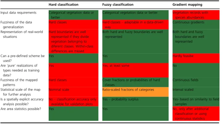
Table 3. Direct comparison of the three mapping approaches. Color-coding: green=offers more flexibility or higher mapping detail, yellow= neutral, red=affected by limitations.

Hard classification Fuzzy classification Gradient mapping

Input data requirements Categorical vegetation data or better

Categorical vegetation data or better Vegetation records with species abundances Fuzziness of the data

generalization

Hard classes Hard classes–adaptable in a data-driven way

Continuous gradients Representation of real-world

situations

Hard boundaries are well represented if they divide vegetation belonging to diferent classes. Within-class differences are missed.

Both hard and fuzzy boundaries are well represented

Can a pre-defined scheme be used?

Yes Yes Hardly feasibe

Are ‘pure’ realizations of types needed as training data?

Yes Yes, at least some No

Fuzziness of the mapped patterns

Hard classes Cover fractions or probabilities of hard classes

Continuous fields Statistical scale of the map

for further analysis

Nominal scale Ratio-scaled fractions of categories Interval scaled Is a spatially explicit accuracy

analysis possible?

No–classification accuracy only available for validation plots

Yes–probability surplus Yes- based on similarity to field samples

Are area statistics possible? Yes Yes No, only after additional

classification or using continuous statistics

(13)

Oldeland and an anonymous reviewer for their comments that helped to improve this paper.

Authors’ contributions

HF and AZ conceived the idea and designed the study with crucial contributions by SSch and GMF. HF sampled the vegetation data, DD and AL designed and conducted the flight campaign and were responsible for image data pre-processing. HF, AK and AZ conducted the analyses.

All authors discussed the results. HF, AZ and SSch led the writing of the paper. All authors contributed substan- tially to the drafts and gave final approval for publication.

Data Availability statement

The data used in this study are archived in the EVA database (http://euroveg.org/eva-database) and the global index of vegetation plot databases (https://www.givd.info, ID EU-DE-037).

References

Binaghi, E., Brivio, P.A., Ghezzi, P. & Rampini, A. (1999) A fuzzy set-based accuracy assessment of soft classification.

Pattern Recognition Letters,20, 935–948.

Breiman, L. (2001) Random forests.Machine Learning,45, 5–32.

Bush, A., Sollmann, R., Wilting, A. et al. (2017) Connecting Earth observation to high-throughput biodiversity data.

Nature Ecology & Evolution,1, 0176.

Clements, F.E. (1916) Plant succession: an analysis of the development of vegetation (No. 242). Carnegie Institution of Washington.

de Klerk, H.M., Burgess, N.D. & Visser, V. (2018) Probabilistic description of vegetation ecotones using remote sensing.

Ecological Informatics,46, 125–132.

Duff, T.J., Bell, T.L. & York, A. (2014) Recognising fuzzy vegetation pattern: the spatial prediction of floristically defined fuzzy communities using species distribution modelling methods.Journal of Vegetation Science,25, 323– 337.

Feilhauer, H., Dahlke, C., Doktor, D., Lausch, A., Schmidtlein, S., Schulz, G. et al. (2014) Mapping the local variability of Natura 2000 habitats with remote sensing.Applied Vegetation Science,17, 765–779.

Feilhauer, H., Doktor, D., Schmidtlein, S. & Skidmore, A.K.

(2016) Mapping pollination types with remote sensing.

Journal of Vegetation Science,27, 999–1011.

Feilhauer, H., Faude, U. & Schmidtlein, S. (2011) Combining Isomap ordination and imaging spectroscopy to map continuous floristic gradients in a heterogeneous landscape.

Remote Sensing of Environment,115, 2513–2524.

Foody, G.M. (1996) Fuzzy modelling of vegetation from remotely sensed imagery.Ecological Modelling,85, 3–12.

Foody, G.M. (1999) The continuum of classification fuzziness in thematic mapping.Photogrammetric Engineering &

Remote Sensing,65, 443–452.

Foody, G.M. (2002) Status of land cover classification accuracy assessment.Remote Sensing of Environment,80, 185–201.

Foody, G.M., Campbell, N.A., Trodd, N.M. & Wood, T.F.

(1992) Derivation and application of probabilistic measures of class membership from the maximum-likelihood classification.Photogrammetric Engineering and Remote Sensing,58, 1335–1348.

Gleason, H.A. (1926) The individualistic concept of the plant association.Bulletin of the Torrey Club,53, 7–26.

Hand, D.J. (2012) Assessing the performance of classification methods.International Statistical Review,80, 400–414.

Khatami, R., Mountrakis, G. & Stehmann, S.V. (2017) Mapping per-pixel predicted accuracy of classified remote sensing images.Remote Sensing of Environment,191, 156– 167.

Kumar, A. & Dadhwal, V.K. (2010) Entropy-based fuzzy classification parameter optimization using uncertainty variation across spatial resolution.Journal of the Indian Society of Remote Sensing,38, 179–192.

Ohmann, J.L. & Gregory, M.J. (2002) Predictive mapping of forest composition and structure with direct gradient analysis and nearest-neighbor imputation in coastal Oregon, USA.Canadian Journal of Forest Research,32, 725–741.

Ohmann, J.L., Gregory, M.J., Henderson, E.B. & Roberts, H.M. (2011) Mapping gradients of community composition with nearest-neighbour imputation: extending plot data for landscape analysis.Journal of Vegetation Science,22, 660–676.

Oldeland, J., Dorigo, W., Lieckfeld, L., Lucieer, A. & J€urgens, N. (2010) Combining vegetation indices, constrained ordination and fuzzy classification for mapping semi-natural vegetation units from hyperspectral imagery.Remote Sensing of Environment,114, 1155–1166.

Pontius, D. (2002) Statistical methods to partition effects of quantity and location during comparison of categorical maps at multiple resolutions.Photogrammetric Engineering

& Remote Sensing,68, 1041–1049.

Rocchini, D. (2010) While Boolean sets non-gently rip: a theoretical framework on fuzzy sets for mapping landscape patterns.Ecological Complexity,7, 125–129.

Schmidtlein, S. & Sassin, J. (2004) Mapping of continuous floristic gradients in grasslands using hyperspectral imagery.

Remote Sensing of Environment,92, 126–138.

Schmidtlein, S., Tichy, L., Feilhauer, H. & Faude, U. (2010) A brute-force approach to vegetation classification.Journal of Vegetation Science,21, 1162–1171.

Schmidtlein, S., Zimmermann, P., Sch€upferling, R. & Weiß, C.

(2007) Mapping the floristic continuum: ordination space

(14)

position estimated from imaging spectroscopy.Journal of Vegetation Science,18, 131–140.

Shanmugam, P., Ahn, Y.H. & Sanjeevi, S. (2006) A comparison of the classification of wetland

characteristics by linear spectral mixture modelling and traditional hard classifiers on multispectral remotely sensed imagery in southern India. Ecological Modelling, 4, 379–394.

Silvan-Cardenas, J.L. & Wang, L. (2008) Sub-pixel confusion– uncertainty matrix for assessing soft classifications.Remote Sensing of Environment,112, 1081–1195.

Tenenbaum, J.B., da Silva, V. & Langford, J.C. (2000) A global geometric framework for nonlinear dimensionality

reduction.Science,290, 2319–2323.

Thessler, S., Ruokolainen, K., Tuomisto, H. & Tomppo, E.

(2005) Mapping gradual landscape-scale floristic changes in Amazonian primary rain forests by combining ordination and remote sensing.Global Ecology and Biogeography, 14, 315–325.

Trodd, N.M. (1996) Analysis and representation of heathland vegetation from near-ground level remotely-

sensed data.Global Ecology and Biogeography Letters,5, 206– 216.

Unberath, I., Vanierschot, L., Somers, B., Van De Kerchove, R., Vanden Borre, J., Unberath, M. & et al. (2019) Remote sensing of coastal vegetation: dealing with high species turnover by mapping multiple floristic gradients.Applied Vegetation Science,22, 534–546.

Wang, F. (1990) Fuzzy supervised classification of remote sensing images.IEEE Transactions on Geoscience and Remote Sensing,28, 194–201.

Wold, S., Sj€ostrom, M. & Eriksson, L. (2001) PLS-regression€ – a basic tool of chemometrics.Chemometrics and Intelligent Laboratory Systems,58, 109–130.

Zadeh, L.A. (1965) Fuzzy sets.Information and Control,8, 338–353.

Zlinszky, A. & Kania, A. (2016) Will it blend? Visualization and accuracy evaluation of high-resolution fuzzy vegetation maps. International Archives of the Photogrammetry, Remote Sensing and Spatial Information Sciences. Prague, Czech Republic: 335–342. 10.5194/isprsarchives-XLI-B2-335- 2016