for radially symmetric solutions of PDEs

Computer-assisted proofs

for radially symmetric solutions of PDEs

Istv´ an Bal´ azs

Jan Bouwe van den Berg

Julien Courtois

J´ anos Dud´ as

Jean-Philippe Lessard

Anett V¨ or¨ os-Kiss

JF Williams

Xi Yuan Yin

Abstract

We obtain radially symmetric solutions of some nonlinear (geometric) partial differ- ential equations via a rigorous computer-assisted method. We introduce all main ideas through examples, accessible to non-experts. The proofs are obtained by solving for the coefficients of the Taylor series of the solutions in a Banach space of geometrically decaying sequences. The tool that allows us to advance from numerical simulations to mathematical proofs is the Banach contraction theorem.

Keywords

Radially symmetric solutions·PDEs·Computer-assisted proofs Taylor series·Contraction mapping theorem

Mathematics Subject Classification (2010) 65M99·65G40·35K57

1 Introduction

In the last decade powerful techniques for turning numerical simulations of ordinary and par- tial differential equations into mathematically rigorous statements have developed rapidly (see e.g. [10, 16, 28, 31, 34, 36]). These methods bridge the divide between scientific computing and abstract mathematical analysis. The foundations for the field were laid in [12, 13, 17]. These methods have received renewed attention due to contemporary computational power as well as

∗MTA-SZTE Analysis and Stochastics Research Group Bolyai Institute, University of Szeged, Aradi v´ertan´uk tere 1, Szeged, Hungary, H-6720. balazs.istvan.88@gmail.com

†VU Amsterdam, Department of Mathematics, De Boelelaan 1081, 1081 HV Amsterdam, The Netherlands.

janbouwe@few.vu.nl

‡Universit´e de Montr´eal, D´epartement de Math´ematiques et de Statistique, Pavillon Andr´e-Aisenstadt, 2920 chemin de la Tour, Montreal, QC, H3T 1J4, Canada. courtoisj@dms.umontreal.ca

§Bolyai Institute, University of Szeged, Aradi v´ertan´uk tere 1, Szeged, Hungary, H-6720. dudas88@gmail.com

¶McGill University, Department of Mathematics and Statistics, Burnside Hall, 805 Sherbrooke Street West, Montreal, Qu´ebec H3A 0B9, Canada. jp.lessard@mcgill.ca

kBolyai Institute, University of Szeged, Aradi v´ertan´uk tere 1, Szeged, Hungary, H-6720.

vorosanett89@gmail.com

∗∗Simon Fraser University, Department of Mathematics, 8888 University Drive Burnaby, BC, V5A 1S6, Canada. jfwillia@sfu.ca

††McGill University, Department of Mathematics and Statistics, Burnside Hall, 805 Sherbrooke Street West, Montreal, Quebec, H3A 0B9, Canada. xi.yin@mail.mcgill.ca

recent algorithmic advances. With a clever hybrid approach one can off-load the verification of intricate computationally intensive estimates to the computer to prove existence to infinite dimensional continuum problems near numerical approximations. This permits using classical ideas (such as fixed point methods) to generate results not accessible by any other means. Thus, going beyond simulations, we can get our hands on solutions of nonlinear (geometric) partial differential equations (PDEs) using the computer and still argue about them with all the rigour of a classical pencil and paper proof.

In this paper we present examples of this technique which we believe are valuable because we prove existence of particular solutions of nontrivial nonlinear PDEs, while the technicalities are minimal (and the associated coding is easily manageable). In particular, we consider two instances of the nonlinear elliptic problem

∆u+f(u) = 0. (1)

In the first type we consideru=u(x) to be scalar with the independent variablexlying in the 2-sphere. In the second type, the unknown u=u(x) is a vector inR² and xlies in the unit disc inR² (with Dirichlet boundary conditions). The specific choices for the nonlinearitiesf will be made explicit in Sections 3 and 4.

When restricting attention to solutions which are invariant under rotation (radially sym- metric solutions), these PDEs reduce to ordinary differential equations (ODEs). The boundary value problems for these nonlinear ODEs are amenable to an approach based on power series.

Numerically one can obtain approximations for finitely many of the Taylor coefficients. To prove that such a truncated series corresponds to a solution of the differential equation, we will apply a Newton-Kantorovich type argument, see Section 2. This not only proves the existence of a solution, but also yields a rigorous bound on the truncation and approximation errors.

Finally, one ingredient that is needed in the analysis in order to control rounding errors, is computation using interval arithmetic. We refer to [21, 24, 29] for an introduction to interval arithmetic. The results in this paper make use of the packageIntlab [23] forMatlab. All matlab scripts are available at [4].

This paper, and in particular the examples discussed, resulted from a three week summer school for undergraduate students at Simon Fraser University in the summer of 2015. During that school, there were exploration sessions for students to investigate the ideas of rigorous computing through exercises and research problems. A small fraction of the students managed to obtain novel results about open problems, and these results constitute the content of the present paper.

2 A Newton-Kantorovich type theorem

When trying to solve numerically a finite dimensional nonlinear zero-finding forF :Rⁿ→Rⁿ, the classical approach is to apply Newton’s algorithm, where one iterates the map

T(x) =x−DF(x)⁻¹F(x),

until the residue gets small. Often this numerical outcome x^num is either assumed “good enough” (roughly, in applied mathematics) or “not rigorous” (roughly, in pure mathematics).

Our goal is to merge these perspectives by providing a rigorous quantitative statement on how good this numerical outcome is, i.e., how close it is to a solution ofF(x) = 0. The crucial observation is that Newton’s method works so well because the map T is a contraction with a very small contraction constant on a neighborhood of a zero x^sol of F, provided that the

JacobianDF(x^sol) is invertible, i.e.,x^sol is a non-degenerate zero ofF (the generic situation).

This allows us toprovethat the numerical approximationx^numis close to the true solutionx^sol. Rather than going into detail about how to obtain such a computer-assisted proof, we first move to the infinite dimensional setting. After detailing in Theorem 2.1 below the setup in gen- eral Banach spaces, we return in Remark 2.2 and Example 2.3 to the (relatively straightforward) application to finite dimensional problems.

Consider nowF :X→X⁰a smooth map between two Banach spaces. A standard approach of mathematical analysis is to turn the zero finding problemF(x) = 0 into a fixed point problem.

The Newton operator itself is usually impractical because the inverse of the derivative of an infinite dimensional map is hard to work with. Instead, one maychoosean injective linear map A∈L(X⁰, X) and study the fixed point problem

x=T(x)^def= x−AF(x).

The main problem is how to chooseAsuch thatT is a contraction on some neighborhood of the (unknown) fixed point that we are looking for. In the context of a computer-assisted proof, the approach is the following. First, by your favorite method from scientific computing, choose a finite dimensional ‘projection’F^numofF, solve it numerically to findx^num, and reinterpretx^num as an element of the infinite dimensional space, which we denoted by ¯x(henceF^num(x^num)≈0 andF(¯x)≈0). We expect the solution to be close to ¯x, hence we would like to choose Aan approximate inverse ofDF(¯x).

How to determine whenAis an appropriately accurate approximate inverse? And on which neighborhood of ¯xdo we get thatT is a contraction? The following theorem is one way to make this precise. It uses, as an intermediate tool, and approximationA^†∈L(X, X⁰) ofDF(¯x).

Theorem 2.1. [Radii polynomial approach in Banach spaces]LetX andX⁰ be Banach spaces. Denote the norm on X by k · k_X. Consider bounded linear operators A^† ∈L(X, X⁰) andA∈L(X⁰, X). AssumeF:X →X⁰ isC¹, thatA is injective and that

AF:X →X. (2)

Consider an approximate solutionx¯ of F(x) = 0(usually obtained using Newton’s method on a finite dimensional projection). LetY0,Z0,Z1, andZ2 be positive constants satisfying

kAF(¯x)kX≤Y0 (3)

kI−AA^†k_B(X)≤Z0 (4)

kA[DF(¯x)−A^†]kB(X)≤Z1, (5) kA[DF(c)−DF(¯x)]k_B(X)≤Z2r, for all kc−xk¯ X≤r, (6) where k · k_B(X) is the induced operator norm for bounded linear operators from X to itself.

Define the radii polynomial

p(r)^def= Z2r²−(1−Z1−Z0)r+Y0. (7) If there existsr0>0 such that

p(r0)<0,

then there exists a uniquex˜∈Br₀(¯x)^def= {x∈X | kx−xk¯ X ≤r0} satisfyingF(˜x) = 0.

Proof. Using the mean value theorem, it is not hard to show that T mapsB_r0(¯x) into itself, and that T is a contraction on that ball with contraction constant κ≤Z₀+Z₁+Z₂r₀ <1.

The result then follows directly from the Banach contraction theorem. We refer to [15] for additional details.

This theorem fits in a long tradition of quantitative Newton-Kantorovich type theorems.

The bounds are parametrized in terms ofr, so that an appropriaterdoes not need to be guessed in advance but rather can be determined as the final step of the proof process. Moreover, it allows us to obtain balls for an interval of values for the radius. Small values ofr0give us the tightest control on the distance between the solution and the numerical approximation, while large values ofr0 provide us with the best information about the isolation of the solution.

Before we show, in Sections 3 and 4 how to apply Theorem 2.1 in practice in infinite dimensional settings, we first come back to finite dimensional problems.

Remark 2.2. In finite dimensions Theorem 2.1 can be implemented very easily and generally, if one has an interval arithmetic package, and if one has explicit formulas forD_jF_i andD²_jkF_i for1 ≤i, j, k ≤n. We use the ∞-norm |x|= max_1≤i≤n|xi|. Letx¯ =x^num be the numerical approximation of a solution (e.g. found using Newton iterations). Let A be a numerical com- puted (hence approximate) inverse of the numerically computedDF(x^num). Now compute with interval arithmeticA^† =DF(x^num), which implies we may set Z₁= 0. Then evaluate, again with interval arithmetic, the following three computable expressions:

1. the residue

Y0= sup

1≤i≤nmax |(AF(x^num))i| ,

where absolute values are taken component-wise, and sup denotes the supremum of the interval obtained.

2. the matrix norm

Z0= sup

1≤i≤nmax X

1≤j≤n

|(I−AA^†)ij|

.

By checking thatZ0<1, one verifies that the hypothesis in Theorem 2.1 thatAis injective.

3. the second derivative estimate (which provides a bound (6) via the mean value theorem) Z2= sup

1≤i≤nmax X

1≤k,m≤n

X

1≤j≤n

AijD²_kmFj x^num+ [−r_∗, r_∗]

,

wherex^num+ [−r_∗, r_∗]is the vector of intervals with components [x^num_k −r_∗, x^num_k +r_∗].

Here we choose a loose a priori upper boundr_∗on the value ofr, and we bound the second derivative uniformly on this ball of radius r_∗.

Since Y0 and Z0 are usually near machine precision, the quadratic formula then gives a very small r0 for whichp(r0)<0. After checking that r0 ≤r∗ we can then invoke Theorem 2.1 to prove that a (unique) zerox^sol ofF lies within distance r0 ofx^num.

Example 2.3. We consider the circular restricted four body problem (CR4BP), where three bodies (with masses(m₁, m₂, m₃), normalized so that m₁+m₂+m₃= 1 andm₁≥m₂≥m₃) move in circular periodic orbits around their center of mass in a triangular configuration that is fixed in the co-rotating frame. A fourth masslesssatellite moves in the effective potential (in this co-rotating frame)

Ω(x, y;m₁, m₂, m₃)^def= 1

2(x²+y²) +

3

X

i=1

m_i

[(x−xi)²+ (y−yi)²]^1/2.

Here (x, y) is the position of the satellite in the plane of the triangle, and the fixed positions (xi, yi)of the three bodies can be expressed in terms of their masses:

(x1, y1) = −^M₂,0

, (x2, y2) = ^K_M^2,3,−

√ 3m3

M

, (x3, y3) = ^K_M^3,2,

√ 3m2

M

,

whereKi,j

def= (m1−mj)mj+ (2m1+mj)mi andM ^def= 2(m²₂+m2m3+m²₃)^1/2, see e.g. [5, 9].

The equilibria of the system are given by the critical points of the effective potentialΩ:

F(x, y)^def= x−

3

X

i=1

mi(x−xi)

[(x−x_i)²+ (y−y_i)²]^3/2, y−

3

X

i=1

mi(y−yi) [(x−x_i)²+ (y−y_i)²]^3/2

!

= 0. (8) It is known that the number of equilibrium points varies from 8 to 10 when the masses are varied (e.g. see [18, 6, 7] and [26]).

Using the general bounds introduced in Remark 2.2 for the finite dimensional case, we applied the radii polynomial approach to prove the existence of several solutions of (8), hence yielding rigorous bounds for relative equilibria of (CR4BP) Let us present a sample result. In case of equal masses m1 = m2 = m3 = 1/3, the routine script equilibria.m, available at [4], computes (using Newton’s method) x^num = (−0.467592983336122,0.809894804400869), and yields the boundsY0= 1.775×10⁻¹⁵,Z0= 1.23×10⁻¹⁴ andZ2 = 12.6987 with the choice of r_∗ = 0.02. In this case, we obtainp(r0)<0 for any r0∈[1.78×10⁻¹⁵,0.02], with pthe radii polynomial defined in (7). In Figure 1 one can find several sample results, where each point has been rigorously validated using the computer program.

-1 0 1

x -1.5

-1 -0.5 0 0.5 1 1.5

y

-1 -0.5 0 0.5 1

x -1

-0.5 0 0.5 1

y

Figure 1: (Left) Ten relative equilibria of (CR4BP) with equal masses. (Right) Eight rel- ative equilibria of (CR4BP) with masses m₁ = 0.9987451087, m₂ = 0.0010170039 and m₃= 0.0002378873. In both plots, some level sets of the effective potential Ω are depicted.

We now turn our attention to the elliptic PDE problems, where we apply Theorem 2.1 in an infinite dimensional setting.

3 Radially symmetric solutions of a nonlinear Laplace- Beltrami operator on the sphere

We consider the partial differential equation

∆u+λu+u²= 0 (9)

posed on the sphereS² ⊂R³, where ∆ is the Laplace-Beltrami operator on the manifold (the natural geometric generalization of the Laplace operator). Hereλ ≥ 0 is a parameter. The PDE (9) describes a classical nonlinear elliptic problem [19], often studied on the unit ball in arbitrary dimension and with a variety of nonlinearities. Here we restrict attention to a quadratic nonlinearity, and we pose the problem on asphere, cf. [11, 33].

Lettingx=rcosφsinθ,y=rsinφsinθ andz=rcosθ, lettingu(x, y, z) =u(r, φ, θ),

∆u= 1

r²sinθ

∂

∂θ

sinθ∂u

∂θ

+ 1

r²sin²θ

∂²u

∂φ².

We look for solutions of (9) that are radially symmetric (with respect to rotations around the z-axis) and symmetric in the equator. This reduces the PDE to an ODE and leads to the following boundary value problem (BVP) foru=u(θ):







u⁰⁰(θ) + cot(θ)u⁰(θ) +λu(θ) +u(θ)²= 0, forθ∈(0,^π₂], u⁰(0) = 0,

u⁰(^π₂) = 0.

(10)

The goal is to prove existence of solutions of (10) via the radii polynomial approach (see Theorem 2.1). The first step in doing so is to introduce a zero finding problem of the form F(x) = 0 on a Banach space.

3.1 The zero finding problem for the Laplace-Beltrami problem

Our approach will be based on Taylor series, and it turns out that it has advantages (see Remark 3.1 below) to work on a domain [0,1]. Hence we rescale the independent variable θ= ^π₂ϑ. The algebra is nicer if we also scale the dependent variable, as well as the parameterλ:

v(ϑ) = π² 4 uπ

2ϑ

and λ˜=π² 4 λ.

The BVP (10) in the new variables becomes











v⁰⁰(ϑ) +π

2ϑcotπ

2ϑv⁰(ϑ)

ϑ + ˜λv(ϑ) +v(ϑ)²= 0 forϑ∈(0,1], v⁰(0) = 0,

v⁰(1) = 0.

(11)

For the sake of presentation, here we have anticipated that it will be convenient to split off a factor ϑ in the second term of the differential equation, as it will allow us to deal with smooth functions that are even inϑonly. We search forv as a power series ofϑaround zero:

v(ϑ) =P∞

n=0anϑⁿ. Let us assume for the moment that the radius of convergence of our power series is larger than 1, then the coefficients are in a Banach space of geometrically decaying coefficients. More precisely, forν >1, denote

`¹_ν ^def= n

a= (a_n)_n≥0:kak_1,ν^def= X

n≥0

|a_n|νⁿ <∞o .

Givena, c∈`¹_ν, denote bya∗cthe Cauchy product given component-wise by (a∗c)n= X

n1 +n2 =n 0≤n1,n2≤n

an₁cn₂ =

n

X

n1=0

an₁c_n−n1.

An important property of the space`¹_νis that it is a Banach algebra under the Cauchy product:

ka∗ck1,ν ≤ kak1,νkck1,ν. (12) The expansion for the cotangent is

cot(θ) = 1 θ−2

∞

X

n=1

θ²ⁿ⁻¹

π²ⁿ ζ(2n), whereζ(2n)^def=

∞

X

k=1

1

k²ⁿ is the Riemann zeta function.

Hence we get

π

2ϑcotπ 2ϑ

= 1−2

∞

X

n=1

ζ(2n) 2²ⁿ ϑ²ⁿ =

∞

X

j=0

bjϑ^j,

where theb_j are the Taylor coefficients defined by b0= 1, bj=−2ζ(j)

2^j ifj≥1 is even, bj = 0 if is odd.

The decay rate of these coefficients shows that we should restrict attention to 1< ν <2. After expanding all terms in (11) as Taylor series, using the Cauchy product, and equating powers, we arrive at the operatorF(a) = (Fn(a))_n≥0 defined as

F_n(a)^def=







a₁ forn= 0,

P∞

j=1jaj forn= 1,

n(n−1)a_n+ (J a∗b)_n+ ˜λa_n−2+ (a∗a)_n−2 forn≥2.

(13)

Here the multiplication operatorJ on sequence spaces is defined by (J a)j

def= jaj forj≥0.

Remark 3.1. Without the rescaling of the independent variable, the formula forF1correspond- ing to the boundary condition atθ= ^π₂ would have becomeP

j≥1jaj(^π₂)^j. Evaluating this sum (say up to some finite N) is numerically unstable because of the high powers of ^π₂. Hence the rescaling.

The following result expresses that to solvingF(a) = 0 leads to a solution of (11).

Lemma 3.2. Let ν ∈(1,2) and let a = (an)_n≥0 ∈ `¹_ν be such that Fn(a) = 0 for alln ≥0.

Thenv(ϑ) =P

n≥0anϑⁿ is a solution of (11).

Proof. Let ν ∈ (1,2) and a ∈ `¹_ν. Then the power series v(ϑ) = P

n≥0anϑⁿ converges uni- formly forϑ∈[0,1], and similarly for the derivatives ofv. The first two equationsF0(a) = 0 andF1(a) = 0 imply that v satisfies the boundary conditions in (11), whereas the remaining equationsFn(a) = 0,n≥2 imply thatv satisfies the differential equation in (11).

Now that we have identified the zero finding problemF(a) = 0 to be solved in the Banach spaceX = `<sup>1</sup><sub>ν</sub> with ν ∈ (1,2) to be chosen later, we are ready to apply the radii polynomial approach as introduced in Theorem 2.1. The first ingredient is a numerical approximation ¯a ofF(a) = 0. Given N ∈ N and a = (an)<sub>n≥0</sub> ∈X =`¹_ν, denote by a^(N) = (an)^N_n=0 ∈ R^N+1 the finite dimensional projection of a, and by F^(N) : R^N+1 → R^N+1 the finite dimensional projection ofF defined by

F^(N)(a^(N))^def= F_n(a^(N),0,0,0, . . .)

0≤n≤N.

Assume that a numerical approximation ¯a^(N) ∈ R^N+1 has been computed. We abuse slightly the notation by identifying ¯a^(N)∈R^N+1with ¯a= (¯a0,a¯1,· · ·,¯aN,0,0,0,· · ·)∈X =`¹_ν. Denote byDF^(N)(¯a) the Jacobian ofF^(N)at ¯a. The radii polynomial approach as introduced in Theorem 2.1 requires defining the operatorsA^† andA. Let

(A^†h)_n^def=

( DF^(N)(¯a)h^(N)

n for 0≤n≤N, n²hn forn > N,

where the diagonal tail is chosen in view of the dominant term in (13) for largen. Consider an (N+ 1)×(N+ 1) matrixA^(N)computed so thatA^(N)≈DF^(N)(¯a)⁻¹. DefineA as

(Ah)n

def=

( A^(N)h^(N)

n for 0≤n≤N,

n⁻²hn forn > N. (14)

It follows thatA is injective whenever the matrixA^(N) is injective, which we verify (see Sec- tion 3.3) in order to check the injectivity assumption in Theorem 2.1. One way to visualize the operatorAis as

A=











A^(N) 0 0 . . .

0 _(N+1)¹ 2 0 . . . 0 0 _(N+2)¹ 2 . . . ... ... ... . ..









 .

The following lemma states that condition (2) of Theorem 2.1 holds.

Lemma 3.3. LetX =`¹_ν withν ∈(1,2),A as in (14)andF as in (13). Then AF :X →X.

We leave the proof to the reader.

We now introduce the formulas for the boundsY0,Z0,Z1andZ2satisfying respectively (3), (4), (5) and (6). These bounds are derived in Sections 3.2–3.5. We first introduce an auxiliary result, used for theZ0 andZ2 bounds. We again leave the proof to the reader (see e.g. [15]).

Lemma 3.4. Consider a linear operatorQ:`<sup>1</sup><sub>ν</sub> →`¹_ν of the form

Q=











Q^(N) 0

qN+1

qN+2

0 . ..











whereQ^(N)= Q^(Nm,n⁾

0≤m,n≤N andq_n ∈R. Assume that|q|_∞= sup_n>N|q_n|<∞. Then kQk_B(`1

ν)= max

0≤n≤Nmax 1 νⁿ

N

X

m=0

|Q^(N)_m,n|ν^m,|q|_∞

.

3.2 The Y

bound

We look for a boundY0 satisfyingkAF(¯a)k1,ν≤Y0. We note that since ¯an= 0 forn > N, we have (¯a∗¯a)n= 0 for alln >2N. Hence, recalling the definition ofAin (14),

kAF(¯a)k1,ν≤

N

X

n=0

(A^(N)F^(N)(¯a))n

νⁿ+

2N+2

X

n=N+1

1

n²|(J¯a∗b)_n+ (¯a∗¯a)_n−2|νⁿ +

∞

X

n=2N+3

1

n²|(Ja¯∗b)_n|νⁿ.

When calculating the finite sums in this expression, computing anybl involves evaluating the zeta function, which is itself an infinite series. We approximate this series by summing finitely many terms and control the remainder via a straightforward integral estimate.

Concerning the final term in the expression above, sinceζ(s) =P∞

k=1k^−s≤P∞

k=1k⁻²=^π₆² for alls≥2, we have|bl| ≤ ^π₃²2^−l for alll≥1. Hence

∞

X

n=2N+3

1

n²|(J¯a∗b)_n|νⁿ=

∞

X

n=2N+3

1 n²

N

X

j=0

|j¯ajb_n−j|νⁿ

≤ 1

(2N+ 3)²

N

X

j=0

|j¯a_j|ν^j

∞

X

n=2N+3

|bn−j|ν^n−j

≤ 1

(2N+ 3)²

N

X

j=0

|ja¯j|ν^j

∞

X

l=N+3

|bl|ν^l

≤ π²kJak¯ 1,ν

3(2N+ 3)²

∞

X

l=N+3

ν 2

^l

= π²kJ¯ak1,ν

3(2N+ 3)² ν

2

^N+3 1 1−^ν₂

def= Ytail.

We thus set Y0

def=

N

X

n=0

(A^(N)F^(N)(¯a))n

νⁿ+

2N+2

X

n=N+1

1

n²|(J¯a∗b)n+ (¯a∗¯a)_n−2|νⁿ+Ytail. (15)

3.3 The Z

bound

LetB^def= I−AA^†. We remark that the tails ofA andA^† are exact inverses, henceBm,n= 0 whenm > N or n > N. Letting

Z0

def= max

0≤n≤N

1 νⁿ

X

0≤m≤N

|Bm,n|ν^m, (16)

we get from Lemma 3.4 thatkI−AA^†kB(`¹_ν)≤Z0. We note that, as in the finite dimensional case in Remark 2.2, it suffices to check thatZ0<1 to infer that the matrix A^(N)is injective, which in turn implies implies that the linear operatorAis injective. In particular, if one finds anr0 >0 for which the radii polynomial p(r) is negative, then we see from (7) thatZ0 <1, hence the injectivity assumption in Theorem 2.1 is then “automatically” fulfilled.

3.4 The Z

bound

We look for a bound A

DF(¯a)−A^† _B(`1

ν) ≤ Z1. Given h ∈ `¹_ν with khk1,ν ≤ 1, we set z^def= [DF(¯a)−A^†]h. For the finite part (0≤n≤N) we see that

z₀= 0, z₁=P

j≥N+1jh_j, and z_n= 0 forn= 2, . . . N.

For the tail, i.e.n > N, we find

z_n=n(n−1)h_n+ (J h∗b)_n+ ˜λh_n−2+ 2(¯a∗h)_n−2−n²h_n. Using the “chain rule” identityJ(h∗b) = (J h∗b) + (h∗J b) we obtain

z_n=n(˜b∗h)_n−(J b∗h)_n+ ˜λh_n−2+ 2(¯a∗h)_n−2,

where ˜bis the sequence defined by ˜b0= 0 and ˜bn=bn forn≥1. Next we estimate kAzk1,ν =

N

X

n=0

N

X

j=0

A^(N)_n,jzj

νⁿ+ X

n≥N+1

1

n²|zn|νⁿ. (17) For anykhk1,ν ≤1, it is a small exercise to show that|z1| ≤ _ν^NN+1⁺¹ provided N+ 1≥(lnν)⁻¹. Hence the first term in (17) is bounded by _ν^N+1N+1

PN

k=0|A^(N_k,1⁾|. For the infinite tail we first estimate

k˜bk1,ν=X

l≥2

|bl|ν^l≤ π² 3

∞

X

n=1

ν² 4

ⁿ

= π²ν² 3(4−ν²)

def= C₁,

kJ bk1,ν=X

l≥2

l|bl|ν^l≤2π² 3

∞

X

n=1

n ν²

4 ⁿ

= 4π²ν² 3(4−ν²)²

def= C2. Then, using the Banach algebra property (12), we find, for anykhk_1,ν≤1,

X

n≥N+1

1

n²|zn|νⁿ≤ C1

N+ 1+ C2

(N+ 1)² + ν²

(N+ 1)²(|λ|˜ + 2k¯ak1,ν).

Hence, with the requirement thatN+ 1≥(lnν)⁻¹, we set Z₁^def= N+ 1

ν^N+1

N

X

n=0

|A^(N)_n,1|+ C₁

N+ 1+ C₂

(N+ 1)² + ν²

(N+ 1)²(|λ|˜ + 2k¯ak1,ν). (18)

3.5 The Z

bound

Letc∈Br(¯a), that iskc−¯ak1,ν≤r. Givenh∈B1(0), note that ([DF(c)−DF(¯a)]h)_n =

(0 forn= 0,1, 2 ((c−¯a)∗h)_n−2 forn≥2, so that

kA[DF(c)−DF(¯a)]kB(`¹_ν)= sup

h∈B₁(0)

kA[DF(c)−DF(¯a)]hk1,ν≤2ν² sup

h∈B₁(0)

kA[(c−a)¯ ∗h]k1,ν

≤2ν² sup

h∈B1(0)

kAk_B(`1

ν)kc−¯ak1,νkhk1,ν≤2ν²kAk_B(`1 ν)r.

Using Lemma 3.4, we get that 2ν²kAk_B(`1

ν)≤Z₂^def= 2ν²max

max

0≤`≤N

1 ν^`

X

0≤k≤N

A^(N)_k,`

ν^k, 1 (N+ 1)²

. (19)

3.6 Computer-assisted proofs

Combining the bounds (15), (16), (18) and (19), we define the radii polynomialp(r) as in (7).

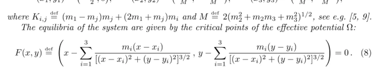
We prove the existence of three different types of solutions by verifying the hypothesis of Theorem 2.1 with the routine script three proofs LB.m available at [4]. The data of each proof can be found in the following table. We find thatp(r)<0 forr∈[r_min, r_max].

solution #1 #2 #3

λ= 4˜λ/π² 5.67 20 19.961

ν 1.06 1.04 1.058

N 250 410 360

Y₀ 4.8014·10⁻⁹ 3.1548·10⁻⁷ 3.9179·10⁻⁷ Z0 4.408·10⁻¹¹ 1.4085·10⁻¹¹ 2.6315·10⁻⁹ Z₁ 4.212·10⁻¹ 2.7293·10⁻² 1.1063·10⁻¹ Z2 7.6773·10³ 4.897·10³ 3.90307·10⁶ r_min 8.3·10⁻⁹ 3.249·10⁻⁷ 5.9684·10⁻⁷ rmax 7.538·10⁻⁵ 1.983·10⁻⁴ 1.6818·10⁻⁶

The three solutions can be seen in Figures 2, 3 and 4. One can observe the different qualitative behaviour of these three solutions.

It is not entirely straightforward to find initial guesses for solutions, i.e., starting points for applying Newton’s method to the finite truncationF^(N). To find such approximate solutions, note that the trivial solutionv= 0 undergoes transcritical bifurcations at ˜λ=π²n(n+¹₂) for n∈ N. The solution branches that bifurcate at these parameter values can then be followed numerically (using branch following techniques) to other parameter values.

The main restriction on the Taylor series based approach presented here, is that not all solutions have an analytic extension to the complex ball of radius 1. These solutions, although real analytic on [0,1], cannot be described by a single Taylor series around the origin. One way to overcome this is via domain decomposition (i.e. matching together several power series), but we will not pursue that here, and it is also by no means the only option.

ϕ

0 0.2 0.4 0.6 0.8 1

v

-2 -1 0 1 2 3 4

Solution #1

Figure 2: (Left) The first solution of (9) on the unit sphereS²⊂R³. (Right) The corresponding (numerical) solution of the BVP (11). Sincer_min<10⁻⁸, the true solution lies with the line- width by Theorem 2.1.

ϕ

0 0.2 0.4 0.6 0.8 1

v

-50 -40 -30 -20 -10 0 10 20

30 Solution #2

Figure 3: (Left) The second solution of (9) on the unit sphere S² ⊂R³. (Right) The corre- sponding (numerical) solution of the BVP (11).

ϕ

0 0.2 0.4 0.6 0.8 1

v

-0.2 0 0.2 0.4 0.6

Solution #3

Figure 4: (Left) The third solution of (9) on the unit sphereS²⊂R³. (Right) The correspond- ing (numerical) solution of the BVP (11).

4 Radially symmetric equilibria of the Swift-Hohenberg equation on the 3D unit ball

We consider the Swift-Hohenberg equation [27] with Dirichlet boundary conditions:

(u_t=−(∆−1)²u+λu−u³, onD₁,

u= ∆u= 0 on∂D1. (20)

Here D1 ⊂ R³ is the unit ball, and λ ∈ R is a parameter. The parabolic PDE (20) is a popular deterministic model for pattern formation, see e.g. [20]. It has been well studied, analytically in one spatial dimension and predominantly numerically in two spatial dimensions.

Here we consider time-independent solutions in three spatial dimensions. Indeed, we will focus on radially symmetric equilibrium solutions of (20). Lettingv= (∆−1)u, these solutions also

correspond to radially symmetric equilibria of the reaction-diffusion system (u_t= ∆u−u−v

vt= ∆v−v−λu+u³ (21)

on the unit ball with Dirichlet boundary conditions. The method works very generally for radi- ally symmetric equilibrium solutions in reaction-diffusion systems (cf. [25]), which are ubiqui- tous in models in the life sciences. This motivates us to work with the system (21) rather than with the equivalent (at the level of equilibria) scalar equation (20). As an additional benefit, the analysis below illustrates how the method of radii polynomials extends naturally to systems of equations. Looking for radially symmetric equilibria of (21), i.e., time independent solutions of the formu(x, y, z) =u(s) =u(p

x²+y²+z²), leads to a coupled systems of ODEs:











u⁰⁰(s) +²_su⁰(s)−u(s)−v(s) = 0 fors∈(0,1], v⁰⁰(s) +²_sv⁰(s)−v(s)−λu(s) +u(s)³= 0 fors∈(0,1], u⁰(0) =v⁰(0) = 0,

u(1) =v(1) = 0.

(22)

We expand the functionsu and v as power series u(s) =P∞

n=0ansⁿ and v(s) = P∞ n=0bnsⁿ. Define the coefficient sequences asa= (an)n≥0andb= (bn)n≥0. Consider the Banach space

X=`<sup>1</sup><sub>ν</sub>×`¹_ν =

x= (a, b) :a, b∈`¹_ν ,

endowed with the normkxkX = max{kak1,ν,kbk1,ν}. The equations for the Taylor coefficients areF1(x) = ((F1(x))n)_n≥0= 0 and F2(x) = ((F2(x))n)_n≥0= 0, given component-wise by

(F1(x))n=







a1 forn= 0,

P

k≥0ak forn= 1,

n(n+ 1)an−an−2−bn−2 forn≥2, (F2(x))n=







b1 forn= 0,

P

k≥0bk forn= 1,

n(n+ 1)bn−b_n−2−λa_n−2+ (a³)_n−2 forn≥2, where

(a³)_n= (a∗a∗a)_n = X

n1 +n2 +n3 =n n1,n2,n3≥0

a_n1a_n2a_n3=

n

X

n1=0

a_n1

n−n1

X

n2=0

a_n2a_n−n1−n2

! .

It is not difficult to derive that all odd coefficients will vanish, but we do not exploit that here.

Denoting F = (F₁, F₂), the problem is to find x= (a, b) ∈ X =`<sup>1</sup><sub>ν</sub> ×`¹_ν for some ν > 1 such thatF(x) = 0. To achieve this, we use the radii polynomial approach as introduced in Theorem 2.1. Given N ∈N, denote x^(N)= ((a_n)_0≤n≤N,(b_n)_0≤n≤N) ∈R^2N+2. Consider the finite dimensional projectionF^(N)= (F₁^(N), F₂^(N)) :R^2N+2→R^2N+2defined by

F_i^(N)(x^(N))^def= (F_i(x^(N)))_k

0≤k≤N.

Given ¯x∈R^2N+2a numerical approximation ofF^(N)(x) = 0, denote byDF^(N)(¯x) the Jacobian ofF^(N) at ¯x, and let us write it as

DF^(N)(¯x) = DaF₁^(N)(¯x) DbF₁^(N)(¯x) DaF₂^(N)(¯x) DbF₂^(N)(¯x)

!

∈R^{(2N+2)×(2N+2)}.

The radii polynomial approach requires defining the operatorsA^† andA. Let A^†= A^†_1,1 A^†_1,2

A^†_2,1 A^†_2,2

!

, (23)

whose action on an elementh= (h1, h2)∈Xis defined by (A^†h)i=A^†_i,1h1+A^†_i,2h2, fori= 1,2.

Here the action ofA^†_i,j is defined as (A^†_i,1h₁)_n=

( D_aF_i^(N)(¯x)h^(N₁ ⁾

n for 0≤n≤N, δi,1n(n+ 1)(h1)n forn > N, (A^†_i,2h2)n=

( DbF_i^(N)(¯x)h^(N₂ ⁾

n for 0≤n≤N, δi,2n(n+ 1)(h2)n forn > N,

whereδi,jis the Kroneckerδ. Consider now a matrixA^(N)∈R(2N+2)×(2N+2)computed so that A^(N)≈DF^(N)(¯x)⁻¹. We decompose it into four (N+ 1)×(N+ 1) blocks:

A^(N)= A^(N_1,1⁾ A^(N_1,2⁾ A^(N_2,1⁾ A^(N_2,2⁾

! .

Thus we defineAas

A=

A_1,1 A_1,2 A_2,1 A_2,2

, (24)

whose action on an elementh= (h1, h2)∈X is defined by (Ah)i =Ai,1h1+Ai,2h2, fori= 1,2.

The action ofAi,j is defined as (Ai,jhj)n=

( A^(N_i,j⁾h^(N_j ⁾

n for 0≤n≤N, δi,j 1

n(n+1)(hj)n forn > N.

As in Section 3.1, to conclude thatAis injective it suffices to check thatA^(N)is injective. The latter is implied by Z0 <1 (see Section 4.2), which is automatically fulfilled when the radii polynomial is negative for somer0>0.

Finally, we setT(x) = x−AF(x), which indeed maps X into itself. As in Section 3, the next step is to derive explicit, computable expressions for the bounds (3), (4), (5) and (6).

4.1 The Y

bound

Observe first that the nonlinear term of F2(¯x) is the Cauchy product (¯a∗¯a∗¯a)_n−2, which vanishes forn≥3N+ 3. This implies that (F1(¯x))n = (F2(¯x))n = 0 for alln≥3N+ 3. For i= 1,2, we set

Y₀^(i)def=

N

X

n=0

2

X

j=1

A^(N_i,j⁾F_j^(N)(¯x)

n

νⁿ+

3N+2

X

n=N+1

1

n(n+ 1)(Fi(¯x))n

νⁿ,

which is a collection of finite sums that can be evaluated with interval arithmetic. We get k[T(¯x)−x]¯ik1,ν=k[−AF(¯x)]ik1,ν=

n

X

j=1

Ai,jFj(¯x) _1,ν

≤Y₀⁽ⁱ⁾,

and we set

Y0

def= max

Y₀⁽¹⁾, Y₀⁽²⁾

. (25)

4.2 The Z

bound

We look for a bound of the formkI−AA^†k_B(X)≤Z0. Recalling the definitions of Aand A^† given in (24) and (23), letB^def= I−AA^† the bounded linear operator represented as

B=

B1,1 B1,2

B2,1 B2,2

.

We remark that (Bi,j)n₁,n₂ = 0 for any i, j = 1,2 whenever n1 > N or n2 > N. Hence we can compute the normskBi,jk_B(`1

ν) using Lemma 3.4. Givenh= (h1, h2)⊂X =`<sup>1</sup><sub>ν</sub>×`¹_ν with khkX = max(kh1k1,ν,kh2k1,ν)≤1, we get

k(Bh)ik1,ν=

2

X

j=1

B_i,jh_{j 1,ν}

≤

2

X

i=1

kBi,jkB(`¹_ν).

Hence we define

Z₀^def= max kB_1,1k_B(`1

ν)+kB_1,2k_B(`1

ν),kB_2,1k_B(`1

ν)+kB_2,2k_B(`1 ν)

. (26)

4.3 The Z

bound

Recall that we look for the boundkA[DF(¯x)−A^†]kB(X)≤Z1. Given h= (h1, h2)∈X with khkX ≤1, set

z^def= [DF(¯x)−A^†]h.

Note that forj= 1,2, (z_j)₀= 0, (z_j)₁=P

k≥N+1(h_j)_k, (z_j)_n= 0 for n= 2, . . . , N, and (z₁)_n=−(h₁)_n−2−(h₂)_n−2, and (z₂)_n =−(h₂)_n−2−λ(h₁)_n−2+ 3(¯a∗a¯∗h₁)_n−2, forn≥N+ 1. It is not hard to show that|(z_j)₁| ≤ν^−(N+1)for allkhk_X ≤1,j= 1,2, hence

k(Az)1k1,ν≤

2

X

j=1

kA1,jzjk1,ν

=

2

X

j=1 N

X

n=0

A^(N_1,j⁾z_j^(N)

n

νⁿ+ X

n≥N+1

1

n(n+ 1)|(z₁)_n|νⁿ

≤ 1 ν^N+1

2

X

j=1 N

X

n=0

A^(N_1,j⁾

n,1

νⁿ+ 1

(N+ 1)(N+ 2)(kh1k1,ν+kh2k1,ν)

≤ 1 ν^N+1

2

X

j=1 N

X

n=0

A^(N_1,j⁾

n,1

νⁿ+ 2 (N+ 1)(N+ 2)

def= Z₁⁽¹⁾,

and similarly, now also using the Banach algebra property (12), k(Az)2k1,ν≤ 1

ν^N+1

2

X

j=1 N

X

n=0

A^(N)_2,j

n,1

νⁿ+ 1

(N+ 1)(N+ 2)(1 +λ+ 3k¯ak²_1,ν) ^def= Z₁⁽²⁾. We thus define

Z1

def= max

Z₁⁽¹⁾, Z₁⁽²⁾

. (27)

4.4 The Z

bound

Letc= (c1, c2)∈Br(¯x), that iskc−xk¯ X = max(kc1−¯ak1,ν,kc2−¯bk1,ν)≤r. GivenkhkX ≤1, note that ([DF1(c)−DF1(¯x)]h)_n = 0 and that

([DF2(c)−DF2(¯x)]h)_n=

(0 forn= 0,1, 3 ((c1∗c1−a¯∗a)¯ ∗h1)_n−2 forn≥2, so that

kA[DF(c)−DF(¯x)]kB(X)= sup

khk_X≤1

kA[DF(c)−DF(¯x)]hkX

≤ kAkB(X) sup

khkX≤1

k[DF(c)−DF(¯x)]hkX

= 3ν²kAk_B(X) sup

khkX≤1

k(c1−a)¯ ∗(c1+ ¯a)∗h1k1,ν

≤3ν²kAk_B(X) sup

khkX≤1

kc1−ak¯ 1,νkc1+ ¯ak1,νkh1k1,ν

≤3ν²kAk_B(X)r(kc₁k_1,ν+k¯ak_1,ν)

≤3ν²kAkB(X)r(r+ 2k¯ak1,ν).

Then, assuming a loose a priori boundr≤1 on the radius, we set Z2

def= 3ν²kAk_B(X)(1 + 2k¯ak1,ν), (28) wherekAkB(X)is computed using Lemma 3.4, see also (26).

4.5 Computer-assisted proofs

With a numerical continuation algorithm, we continued a branch of solutions of (22) that bifurcates from the zero solution atλ= (π²+ 1)². Combining the bounds Y0, Z0,Z1 andZ2

given in (25), (26), (27) and (28), respectively, we define the radii polynomialp(r) as in (7).

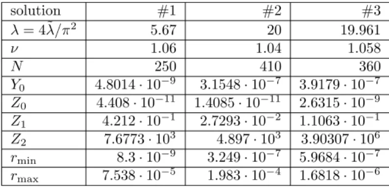
We prove the existence of six solutions of (22) by verifying the hypotheses of Theorem 2.1 with the routinescript proofs SH.m available at [4]. The following table contains values of the bounds, as well as intervals [r_min, r_max] on whichp(r)<0, for sample values ofλranging from 118.2 to 500.

λ ν N Y0 Z1 Z2 rmin rmax

118.2 1.15 39 8.4414·10⁻¹¹ 0.44499 1.9642·10⁶ 1.5218·10⁻¹⁰ 2.8242·10⁻⁷ 120 1.1 54 1.3132·10⁻⁹ 0.15775 2.002·10⁵ 1.5598·10⁻⁹ 4.2056·10⁻⁶ 250 1.04 114 4.3386·10⁻⁸ 0.27014 4.89752·10⁵ 6.2026·10⁻⁸ 1.4282·10⁻⁶ 350 1.03 136 4.8408·10⁻⁸ 0.15617 1.536768·10⁶ 6.508·10⁻⁸ 4.8401·10⁻⁷ 450 1.02 164 4.7337·10⁻⁸ 0.033858 3.274572·10⁶ 6.2042·10⁻⁸ 2.33·10⁻⁷ 500 1.009 169 5.6167·10⁻⁸ 0.06321 3.73724·10⁶ 9.9273·10⁻⁸ 1.5139·10⁻⁷

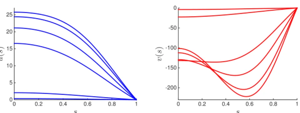
We observe from these data that as we increase the parameter λ, the dimension of the projection N needs to increase while the decay parameter ν needs to decrease. This is due to the fact that the Taylor coefficients of the solutions decay slower asλincreases. Moreover, notice that the values ofr_min and r_max are approaching each other, meaning that the proofs are getting harder and harder to obtain. This suggests that for larger parameter values a single Taylor expansion is not enough. The corresponding solutions can be seen in Figure 5. We plot in Figure 6 the solution (u, v) of (20) atλ= 500.

s

0 0.2 0.4 0.6 0.8 1

u(s)

0 5 10 15 20 25

s

0 0.2 0.4 0.6 0.8 1

v(s)

-200 -150 -100 -50 0

Figure 5: Six solutions of (22) forλ∈ {118.2,120,250,350,450,500}.

s

0 0.2 0.4 0.6 0.8 1

u(s)

0 5 10 15 20 25

Figure 6: (Left) A stationary solution of the Swift-Hohenberg equation (20) on the unit ball inR³at λ= 500. (Right) The corresponding graph ofu(s) =u(p

x²+y²+z²).

5 Conclusion

We have seen that some nontrivial boundary value problems originating from nonlinear (geo- metric) PDEs can be solved in a Taylor series setting, one that requires relatively little technical machinery. Cutting of the Taylor series at some finite order and solving the associated finite di- mensional algebraic system numerically, leads to an approximate solution, and we have proven that the true solution lies nearby. Indeed, based on Theorem 2.1 and computable bounds (us- ing interval arithmetic), we can estimate the distance between approximate and true solution rigorously and explicitly. This turns the numerical computation into a mathematical statement about the PDE.

There are limitations to the particular choice of Taylor series as our means of describing a solution, i.e., using monomials as our basis functions. In particular, we have seen that this puts limits on the parameter range where we can apply this approach. More generally, there is a large variety of functional analytic setups and numerical algorithms, adapted to the particular problem under study, which fit into the general framework of Theorem 2.1. Successful examples include domain decomposition, Fourier series, Chebyshev series, splines, finite elements, as well as combinations of these. With these tools one is able, using the paradigm illustrated by the