Energy Efficiency Analysis of Water and Wastewater Utilities Based on the IBNET Database

Energy Efficiency Analysis of Water and Wastewater Utilities Based on the IBNET

Database

Regional Centre for Energy Policy Research

Corvinus University of Budapest

Client:

The World Bank IBNET Program

Prepared by: REGIONAL CENTRE FOR ENERGY POLICY RESEARCH

Mailing address:1093 Budapest, Fővám tér 8, Hungary Office:1092 Budapest, Közraktár utca 4-6, Room 707.

Phone:+36 1 482-7070Fax:+36 1 482-7037

Email:rekk@uni-corvinus.hu

May 2010 Authors:

Márta Bisztray *, András Kis *, Balázs Muraközy **, Gábor Ungvári *

* Regional Centre for Energy Policy Research, Water Economics Unit

** Institute of Economics, Hungarian Academy of Sciences

Table of Contents

1. Introduction ... 1

2. Literature Review ... 4

2.1 The Role of Operating Conditions on Energy Use ... 4

2.2 Potential Measures to Improve Energy Efficiency ... 6

3. The Data Used ... 9

3.1 IBNET Data ... 9

3.2 Electricity Consumption ... 12

3.3 Terrain ... 13

4. Descriptive Statistics ... 15

5. Regression analysis ... 18

5.1 Methodology ... 18

5.2 Results ... 19

6. Interpretation of the Results ... 25

7. List of Sources ... 33

8. Annex on Data Cleaning ... 35

1

I. INTRODUCTION

Electricity expenditures make up a large part of the operating costs of the water and wastewater sector. In case of the Central and Eastern European (CEE) and Commonwealth of Independent States (CIS)¹ utilities within the IBNET database², for half of the companies electricity costs comprise at least 18% of all operating costs, and for more than one-fifth of the companies electricity costs make up over 30% of all operating costs (Figure 1). Given the large share of these expenditures and the poor financial position of many of these companies, any reduction in electricity costs would be a well appreciated development.

Figure 1. Electricity costs as a percent of all operating costs, CEE and CIS water utilities

0%

10%

20%

30%

40%

50%

60%

70%

80%

1 100

Percent of companies Electricity costs as a percent of all operating costs

Source: IBNET database

Energy costs can be reduced in one of two ways:

1. Lower the unit cost of energy purchases/input.

2. Improve the energy efficiency of operations, i.e. consume less energy for the same amount of production.

There are multiple solutions to reduce the unit cost of electricity. In case of competitive electricity markets it makes sense to pay special attention to the procurement process in order

1 Countries which were part of the Soviet Union were assigned to CIS, all other countries, including Turkey, are considered as CEE as part of this analysis.

2

to attain attractive rates. If the price of electricity changes within the day (as is the case for large consumers in most developed electricity markets), then water utilities can shift some of their consumption to hours with lower electricity tariffs through clever planning and active process control and automation – there is a large and growing body of experience in this field.

Sometimes own generation of electricity is cheaper than purchase from the market.

Production of heat and electricity from sewage sludge is a typical option, but there are some other, more exotic technologies as well. For example, according to Armar and da Silva Filho (2003), some of the water utilities in Brazil started to generate power from micro-hydro plants installed at water intake points. Since only economic investments were implemented, the overall energy costs were also reduced.

While the room for lower unit costs clearly exists - especially as electricity markets open up, multiple intra-day rates of electricity are introduced and the cost of renewable technologies drops -, the cost saving potential from improved energy efficiency is likely to be much higher.

Therefore within the current document we will not address the unit costs of electricity purchases, but nevertheless would like to emphasize that this topic should be part of any reasonable water utility energy strategy. Hereafter we will focus our attention solely on the energy efficiency of water and wastewater utilities.

Improvements in energy efficiency are widely available, as suggested by field experience as well as research findings from all over the World. In the United States potential energy savings of 15-30 percent are "readily achievable" in many water and wastewater plants with substantial financial returns with payback periods of only a few months to a few years³. Given the condition of water and wastewater infrastructure in CEE and CIS we think that similar or higher improvements are feasible for most utilities, especially in lower income countries. Evidence of water supply retrofit schemes from Brazil, another economy in transition, supports these assumptions.

A straightforward way to see how energy efficient a company is compared to its peers is to compute one or more simple indicators. Such a benchmarking exercise is fairly easy to do, but one should be cautious of its results. It is well known that the value of energy efficiency indicators (e.g. kWh of energy used to deliver a cubic meter of drinking water) depends on external operating conditions as much as on company practices. A good value may be an indication of a well maintained, efficient technology – or a flat terrain with moderate need for

2 www.ib-net.org

3 http://www.epa.gov/waterinfrastructure/energyefficiency.htm

3

pumping. Sophisticated indicators can help to account for external conditions. Considering the difference in elevation for a given volume of transported water is a good way to incorporate such exogenous factors. The problem with these indicators is that they require specific detailed data, which is almost never readily available.

Alternatively, if there is a large database of water utility data, we can use statistical techniques to screen for the impact of operating conditions, assuming that the remaining difference between utility indicator values is up to differences in efficiency. Multiple variable statistical analysis of energy efficiency has been successfully applied in the water utility sector (e.g.

Carlson (2007), Bisztray (2009a)). For a comprehensive review of studies focusing on productivity and efficiency see Abbott and Cohen (2009).

The IBNET database includes basic performance data of a large number of water utilities. Our purpose with the study is to see if it is possible to identify the role of operating conditions on the energy efficiency of utilities, using multiple variable statistical analysis. If we are successful then the ensuing results will have wide applicability, including the uses listed below:

 Utility managers often have an opinion on the magnitude of energy saving potential at their firm. The results from the analysis could confirm or disprove their views, and also help them set targets for reduction of energy use.

 Of a group of companies it becomes possible to select the ones with the largest room for energy efficiency improvement. This is valuable input for government policy, national and international aid programs, or banks/institutions providing financing to the sector.

 One of the worthwhile goals of benchmarking projects is exchange of best practices. The results of the described analysis will help to better select those companies which are likely to be good source of best practice information.

4

II. LITERATURE REVIEW

The chapter on literature review has been split in two. The first section provides a glimpse of the operating conditions that past studies have identified as material to the energy use of water and wastewater utilities. This information has been important in shaping our own statistical models and helping to judge the comprehensiveness of our work regarding the coverage of key variables. The second part of the literature review provides a brief overview of the measures that underperforming utilities can apply in order to lower their energy consumption.

II.1. The Role of Operating Conditions on Energy Use

We have studied a number of reports dealing with the internal and external factors shaping the energy use of water and wastewater utilities. In this section we review the key exogenous factors that have been found to have an impact on energy use. For each factor we will describe if the variable in question is also part of the IBNET database, and if not, if we have been able to approximate the missing variables from other sources and methods.

Larger utilities on average require less energy to pump a unit of water, in other words, economies of scale exist (Elliott et. al., (2003), Bisztray et. al. (2009b), Byrnes et. al. (2009) all confirmed this finding). Within the IBNET database size can be represented by multiple variables, including the volume of water sold and wastewater collected.

Both the source of raw water and the treatment applied to it can make substantial differences in energy use. Groundwater extraction from deep aquifers requires substantially more energy than extraction of surface water. Some of the advanced drinking water treatment technologies, such as ozone disinfection and membrane filtration are energy intensive (Elliott et. al., 2003).

Bisztray et. al. (2009b) in their analysis assigned drinking water treatment technologies into one of two categories (“inexpensive” and “expensive”) based on the opinion of utility experts.

Their analysis indicates that Hungarian utilities applying expensive technologies to treat at least 10% of their drinking water face on average 0.13 EUR/m³ higher costs than the rest of the companies. How much of this exactly is due to higher electricity use has not been investigated, but utility experts confirmed that more expensive technologies are also more likely to be energy intensive. Since data on water bases and drinking water treatment

5

technologies is not available within the IBNET database, this factor is not investigated in the present study.

Terrain is also a key factor in explaining energy use. Hungarian utilities operating in hilly areas, categorized as a service area with larger variation in altitude above sea level, use on average 0.65 kWh/m³ more energy for water and 0.2-0.6 kWh/m³ more for wastewater than companies from flat areas (Bisztray et. al. 2009b). The IBNET project does not collect data on the terrain, but knowing the location of the main cities of each utility, it has been possible to generate a proxy for terrain (Chapter III.3).

The AWWA Research Foundation undertook a project to develop energy benchmarking indicators for water and wastewater utilities (Carlson and Walburger, 2007). Since the researchers did not have to work from an existing database, but developed their own survey instruments, it became possible to test the role of a wide spectrum of previously untested variables. Data from 266 wastewater treatment plants and 125 water utilities was statistically analysed. The analysis showed the value of process level benchmarking, i.e. creating separate models for drinking water treatment, drinking water delivery, sewage collection and sewage treatment, and possibly also for sub-processes, using detailed data tailored especially for the process in question. Landon (2009) and Gay Alanis (2009) also emphasize the important contribution that process level benchmarking can make.

Listed below are the key variables that according to the results of Carlson and Walburger (2007) are important drivers of energy efficiency at the process level. The majority of the described data is not available within the IBNET database, therefore process level analysis as part of the current project is not feasible.

 For drinking water delivery total volume, pumping horsepower, the length of distribution mains, network loss and change in elevation through the network played a key role. Of these variables, volume, the length of the distribution mains, and network loss are available in the IBNET database and can therefore be tested in our analysis.

 For drinking water treatment specific technologies – such as oxidation, iron removal, direct filtration and ozone treatment – proved to be important determinants of energy use.

Drinking water technologies are not part of the IBNET survey.

 For sewage collection, besides volume, the pumping horsepower and the number of pumps proved to be important input variables. Pumping data is not collected as part of the IBNET exercise.

6

 For wastewater treatment the following variables substantially impacted energy use:

volume of inflowing wastewater, BOD removal, nutrient removal, capacity utilization, application of trickle filtration. Of these, only volume of wastewater is part of IBNET.

 In case utilities are scattered through a large geographical area, weather may also

influence energy use, through differing needs for heating or cooling. Weather data is not part of the IBNET database and while such information could be assembled, we decided to skip it as there are a number of more important drivers of energy use which are already part of our analysis.

II.2. Potential Measures to Improve Energy Efficiency

Once an analysis identifies the utilities which are likely to have the largest room for energy efficiency improvements, the question that comes to mind is “what can be done to actually lower energy use?”. While answering this question is not among the original goals of our current research, we would like to provide a brief review of the options often cited in literature and guide the reader to some of the valuable reports dealing with this topic.

Before we review the measures, let us provide two general comments:

 Often utility managers are aware of many of their energy saving options, but a full review is best attained through energy audits involving independent experts with experience in water and wastewater utility technologies. Learning from best performing water companies can nicely supplement energy audits.

 Not all energy saving measures are cost-effective to the same extent. A lot of investments will have an attractive pay-back period, while others will take a long time to become self-financing. Managers of utilities with scarce resources are not likely to pursue investments with poor financial returns, but nevertheless, it is good to remember that energy saving investments - or any investments aimed at cost savings -, should ideally be done in an order based on some measure of financial return, like internal rate of return. Multi-purpose investments, which besides energy efficiency also target e.g. more secure supply or better quality drinking water, should obviously be decided on using multiple criteria, financial returns being one of them.

7 Leakage Reduction

According to Raucher, et. al. (2008) annually an estimated 5-10 TWh of electricity is used to pump water which is eventually lost from the networks in the United States. Some of the CEE utilities face drinking water network loss ratios well above 40%. Cutting leakage will reduce the amount of pumped water and therefore the energy need for pumping. Modern technologies can identify the network sections with the biggest savings potential, network remediation should obviously start at these locations.

Improved Pumping

Ijjaz-Vasquez (2005) describes that in the countries of the former Soviet Union about 95% of the energy use of water utilities is attributed to pumping operations. This is the result of large network losses as well as inefficient pumping facilities, due to old age, poor design and improper size. Pumps are often oversized, especially in places where water consumption fell due to increased prices and changes in the economy, and therefore are less efficient when pumping lower volumes of water. Replacing old pumps with more energy efficient devices not only saves energy, but in many cases it will also save maintenance costs and ensure more reliable service. Sometimes it is enough to refurbish existing pumps. These investments often have a short repayment period. As an example, Armar and da Silva Filho (2003) cites two case studies in Brazil in which it was determined that 20 and 30 percent of pumps needed some sort of intervention, resulting in reduced energy use of 5-6 percent. In case pumps are replaced, long-term forecasting of water consumption can aid in selecting energy efficient pumping technology (Jentgen et. al., 2007). The USEPA (2008) recommends that variable frequency driver pumps are considered, as these can adjust to flow volumes and therefore save energy during low volume periods.

Sophisticated Control Systems

There are many novel processes taking advantage of recent technical developments in the field of information technology, engineering, biotechnology and others, which contribute to enhanced operations and energy savings at water and wastewater utilities. While we mention some of these here, our list is far from complete, but should be sufficient to illustrate the wide range of new applications.

Remote sensing and controlling of water flows and pressure helps to avoid excess network pressure, contributing to energy savings in two ways. On the one hand, lower pressure

8

requires less pumping, and on the other, lower pressure results in less leaked water, which in turn also requires less pumping. Intraday forecasting of water consumption and related water flows can be useful in optimizing operation, by utilizing higher efficiency pumps over lower efficiency pumps (Jentgen et. al., 2007). Haecky and Perco (2009) report that replacement and modernization of the aeration system of a wastewater treatment plant in Granollers, Spain resulted in energy savings of 30% for the technology, which is the main energy user within the plant.

9

III. THE DATA USED

III.1. IBNET Data

The CEE and CIS sections of the IBNET database were used for the analysis. The database was cleaned in two steps:

First the whole database was checked for consistency, regardless of whether a specific variable would then be used as part of the current energy efficiency analysis. Raw data were scrutinized for errors, and erroneous data was corrected when feasible, or labelled as missing otherwise. Details about this process are provided in the Annex.

Next, the database was further cleaned specifically to satisfy the data need of the econometric analysis of the present project. Details of this exercise are provided below.

Our main goal with data cleaning was to delete firms where reported data may be distorted.

Also, we tried to restrict the sample to possibly similar firms to estimate a „reasonable practice‟, if not a „best practice‟ electricity use function – we wanted to estimate the technological relationships for the average firm in the region. While it is possible to predict electricity consumption for firms outside the „reasonable practice‟ sample, firms far away from the average technology should not modify the estimated relationships.

We dropped all firms where data about electricity consumption was missing because electricity cost was 0 or there was no data on electricity prices. Unfortunately, a large number of firms did not report electricity consumption in the IBNET database. In Belarus, Tajikistan and Uzbekistan none of the firms had electricity consumption data due to difficulties accessing good quality electricity price data from these countries, while a large share of observations are lost in Albania, Bosnia and Herzegovina, the Kyrgyz Republic and Slovakia.

Altogether more than 100 firms are lost because of missing electricity use data.

We dropped firms which were involved in other possibly energy intensive activities like construction and transport, as it is impossible to estimate the amount of electricity consumed by these other activities. Theoretically these activities are excluded from the reported electricity cost, but we wanted to be on the safe side, especially, as there were only less than 100 firms dropped.

10

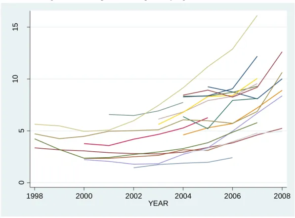
We dropped all years before 1998, as the data on electricity prices was unreliable before this.

Even in 1998 and 1999, electricity prices are declining in USD terms, but this decline does not seem to be very important from the perspective of the analysis. Country-level electricity data is shown in Figure 2.

Figure 2. Non-residential electricity prices, including taxes and excluding VAT, annual average values computed from quarterly figures, USD cent/kWh

051015

Price of electricity, USD cent/kwh

1998 2000 2002 2004 2006 2008

YEAR

From our main estimation sample we dropped firms which were not involved in both water and wastewater services. Firms involved in only one of these activities are few, thus it is not easy to estimate a production function for them with any precision. We also dropped firms where the water production exceeded wastewater collection by a factor of 5 and vice versa.

We, however, also estimated a flexible form relationship on the pooled sample of firms providing either service to be able to predict the electricity use for all firms.

We also dropped outliers with respect to energy efficiency. For this we used a simple rule of thumb: we calculated relative electricity use as electricity (in kWh) over the sum of water and wastewater (in 1000 m³). We dropped firms for which this figure was below 50 or above 5000.

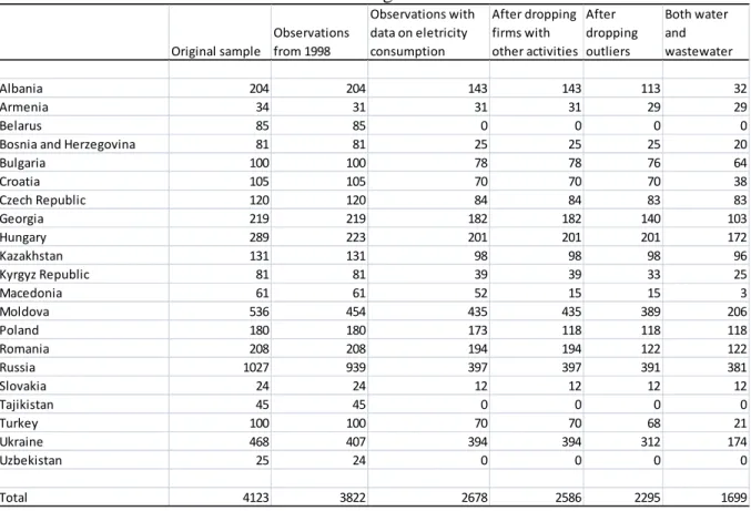
Table 1 shows how the cleaning procedure narrowed the sample step-by-step.

11 Table 1 Number of observations after cleaning

Original sample

Observations from 1998

Observations with data on eletricity consumption

After dropping firms with other activities

After dropping outliers

Both water and wastewater

Albania 204 204 143 143 113 32

Armenia 34 31 31 31 29 29

Belarus 85 85 0 0 0 0

Bosnia and Herzegovina 81 81 25 25 25 20

Bulgaria 100 100 78 78 76 64

Croatia 105 105 70 70 70 38

Czech Republic 120 120 84 84 83 83

Georgia 219 219 182 182 140 103

Hungary 289 223 201 201 201 172

Kazakhstan 131 131 98 98 98 96

Kyrgyz Republic 81 81 39 39 33 25

Macedonia 61 61 52 15 15 3

Moldova 536 454 435 435 389 206

Poland 180 180 173 118 118 118

Romania 208 208 194 194 122 122

Russia 1027 939 397 397 391 381

Slovakia 24 24 12 12 12 12

Tajikistan 45 45 0 0 0 0

Turkey 100 100 70 70 68 21

Ukraine 468 407 394 394 312 174

Uzbekistan 25 24 0 0 0 0

Total 4123 3822 2678 2586 2295 1699

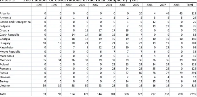
Table 2 shows how observations are distributed over time in the final sample (including firms which provide either water, wastewater or both services). Few countries reported in 1998 and 1999, and some countries did not report in 2008. We have data on all countries with the exception of Croatia in 2005, so we report comparative tables for this year (and 2004 for Croatia).

12

Table 2 The number of observations in the final sample by year

1998 1999 2000 2001 2002 2003 2004 2005 2006 2007 2008 Total

Albania 0 0 0 0 0 0 0 20 4 46 43 113

Armenia 1 1 1 1 1 2 2 5 5 5 5 29

Bosnia and Herzegovina 0 0 0 0 0 0 1 6 12 6 0 25

Bulgaria 0 0 0 0 0 0 2 18 19 19 18 76

Croatia 0 0 0 18 17 17 18 0 0 0 0 70

Czech Republic 0 0 14 14 16 16 16 7 0 0 0 83

Georgia 0 0 18 18 19 19 19 17 10 10 10 140

Hungary 18 18 20 21 21 21 22 22 19 19 0 201

Kazakhstan 0 0 7 9 12 13 16 18 0 23 0 98

Kyrgyz Republic 0 0 0 0 6 7 7 7 6 0 0 33

Macedonia 0 0 0 0 0 0 3 4 4 4 0 15

Moldova 35 34 36 32 29 37 39 36 36 36 39 389

Poland 0 0 0 0 0 23 23 24 24 24 0 118

Romania 0 0 0 0 0 23 24 25 25 25 0 122

Russia 0 0 0 0 0 0 77 80 78 77 79 391

Slovakia 0 0 0 0 0 0 2 2 4 4 0 12

Turkey 0 0 0 0 0 0 14 15 15 18 6 68

Ukraine 39 39 58 59 23 23 23 16 16 16 0 312

Total 93 92 154 172 144 201 308 322 277 332 200 2295

III.2. Electricity Consumption

The IBNET survey collects data on electrical energy costs, but not on energy consumption.

Electricity consumption was estimated by dividing the energy cost with the commercial price of energy. Data on energy prices was obtained either from the Energy Regulators Regional Association (ERRA) database, or the Eurostat Industrial Electricity Price database. For Belarus, Tajikistan and Uzbekistan we did not have a chance to get hold of good quality electricity price data therefore these countries were omitted from the analysis. Electricity prices were checked both across countries and years, to ensure that the database as a whole is consistent.

We believe that the generated dataset for electricity use is of good quality, but we are also well aware that further improvements could be made. To put our data into context, below we list some of the additional improvements – beyond the scope of the current analysis - that could lead to an even better database of electricity use:

 In some wastewater treatment facilities the sewage sludge is anaerobically digested and the resulting biogas is combusted to produce energy. This energy is in most cases used within the facility, satisfying part or all of the energy needs of the sewage treatment plant, and sometimes there is a surplus which is sold to the electricity grid. Biogas generated electricity used within the water and wastewater utility reduces the amount that needs to

13

be purchased from the grid, therefore ideally this amount should be added to the

purchased quantity of electricity. The energy use adjusted this way may in some cases be 10-15 percent higher than reported energy purchases. Power generation from biogas is a relatively new technology in the region, with a low rate of penetration therefore the results of our analysis are not likely to be materially affected by not accounting for it.

 Results of the analysis could probably be notably improved if electricity use was possible to estimate separately for the water and wastewater services. While we did not have a chance to do so, we applied econometric models which make an attempt to separate the impacts of the two services on total energy use. As it is clear from the literature review in Chapter II.1, analyzing process level energy use would make results even more accurate.

 If drinking water is purchased from an external source, less energy will be required on the part of the utility since the purchased water has already been extracted and treated.

Likewise, bulk drinking water sold will carry an intrinsic energy content with it. Having data for the bulk drinking water sales it has been possible to separate the latter impact, but not the former one. Therefore companies buying a large share of their delivered drinking water from other utilities are likely to exhibit better energy efficiency than their true conditions.

 Ideally, all utility energy use should be converted to source energy use - with the possible exception of transport fuel -, as there is some variation of energy inputs among utilities.

This issue was not possible to address within the current piece of research, lacking data on other energy uses, but we assumed that the overwhelming majority of energy use at the water utilities of the region is electricity.

III.3. Terrain

As our earlier analysis (Bisztray et. al., 2009b) of water and wastewater utilities in Hungary indicates, differences in topology among utilities drive some of the difference between the unit costs of operation and also some of the difference between the unit electricity use of water and wastewater services at different companies. In this research terrain was numerically represented by the standard deviation of the altitude above sea level of each settlement within the service area. We also aimed to grasp the geographical differences of the IBNET sample of waterworks to test the relation between terrain and energy use. As we lacked information on

14

the spatial attributes of the service areas of the utilities within the IBNET database, we employed two methods to get a proxy for topology.

The first approach approximates terrain with the altitude above sea level of the main settlement of the service area. Essentially, we assumed that plain areas are more common at lower altitudes, while higher values indicate a mountainous environment with bigger altitude differences inside the service area.

With the second approach we generated a variable which measures the differences in altitude among eight points of the service area. A specific distance, determined by the estimated size of the service area based on the number of settlements, people served and population density⁴, was measured from the center of the main city to eight directions (North, North-East, East etc.) and the altitude above sea level for these eight points was determined. Since population density was not computable for towns with less than 100,000 inhabitants, for these settlements an average value was used based on randomly available population density data from a number of locations.

4http://unstats.un.org/unsd/demographic/products/dyb/dyb2007/Table08.xls

15

IV. DESCRIPTIVE STATISTICS

In this section we report descriptive results using a proxy for energy efficiency – assuming simply that each cubic meter of water or wastewater requires the same amount of electricity.⁵ This variable is calculated as electricity use/(water sold + wastewater quantity); its unit of measurement is kWh/1000 m³. Figure 3 shows the average of this efficiency measure for different countries in 2005.

Figure 3. Median electricity consumption in kWh/1000 m³

0 500 1,000 1,500 2,000

Median electricity consumption, KWH/1000 m3 Ukraine

Turkey Slovakia Russia Romania Poland Moldova Macedonia Kyrgyz Republic Kazakhstan Hungary Georgia Czech Republic Croatia*

Bulgaria Bosnia and Herzegovina Armenia Albania

* for 2004

This graph shows large differences across countries, with larger efficiency on average in higher income countries. Albania and Moldova are strong outliers with exceptional negative performance according to this measure, followed by Slovakia (note that we have only two observations for Slovakia in 2005), Russia and Bosnia-Herzegovina. At the other end of the scale, Georgia, Croatia and the Czech Republic are the most efficient by this simple calculation.

5 From other sources we are aware that this is rarely the case, but did not want to use an arbitrarily picked ratio especially as the difference among the countries of the region is likely to be substantial.

16

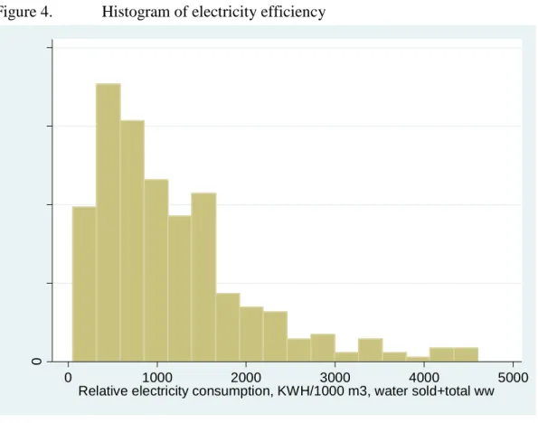
Second, we report the histogram of the proxy for electricity efficiency in 2005 in Figure 4, which suggests that there are large differences in terms of energy efficiency in the CEE and CIS region.

Figure 4. Histogram of electricity efficiency

0

2.0e-044.0e-046.0e-048.0e-04

Density

0 1000 2000 3000 4000 5000

Relative electricity consumption, KWH/1000 m3, water sold+total ww

The next question is whether efficiency and technology is determined by country level variables, or there is important within-country dispersion. To shed some light on this question, we calculated the standard deviation for this measure for each country, which we report in Figure 5.

17

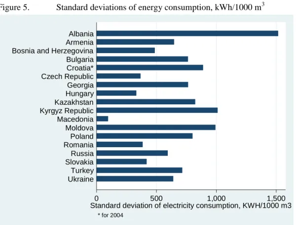
Figure 5. Standard deviations of energy consumption, kWh/1000 m³

0 500 1,000 1,500

Standard deviation of electricity consumption, KWH/1000 m3 Ukraine

Turkey Slovakia Russia Romania Poland Moldova Macedonia Kyrgyz Republic Kazakhstan Hungary Georgia Czech Republic Croatia*

Bulgaria Bosnia and Herzegovina Armenia Albania

* for 2004

The graph reveals that there are large deviations across utilities within countries. On average, these standard deviations are large compared to the median values: for the typical country, the median is about 800 kWh/m³, while the standard deviation is between 300 and 500 kWh/m³. The largest within-country variation is reported in Albania, but in general, within-country standard deviation tends to be larger in CIS and Southern European countries than in the rest of CEE. These numbers suggests that electricity use is not only determined by country-level conditions but individual service providers may improve their performance to a significant degree if they adopt the best practice in their respective countries, especially in CIS and Southern European countries.

18

V. REGRESSION ANALYSIS V.1. Methodology

Next, we apply regression analysis to estimate the determinants of energy efficiency.

Our model follows a cost function approach. In this approach we assume that the electricity need of the firm is determined by the quantity of water and wastewater provided by the firm:

(1)

Where i denotes firms, t denotes the time period, is the quantity of electricity consumed by the firm, is the water provided by the firm, is wastewater collected by the firm, and are the elasticity of electricity use with respect to water and wastewater provision, respectively. If , then increasing returns to scale are present: doubling both water and wastewater quantity requires less than doubling the electricity use. shows the energy efficiency of the firm: the smaller this number, the less electricity the firm consumes per unit of water and wastewater provided. denotes the error term of the regression.⁶

Note that we implicitly assume that technology is similar for all firms in the sample, in the sense that the elasticities, and in it are the same for all firms, and firms only differ in their efficiency. As the empirical analysis shows, country-by-country estimation suggests that this is the case.

When estimating, we take the natural logarithm of both sides of the equation:

(2)

In the following we assume that the energy efficiency term is a function of different variables, e.g. nature of service area, population density, country dummies. Thus when we are interested in the effect of population density on efficiency, we assume that

6 We experimented with other functional forms, but this proved to be the most stable.

19

: efficiency is a (stochastic) function of population density. By substituting this to (1), we estimate:

(3)

Here shows the relationship between population density and energy efficiency. A negative sign of the parameter reflects that energy efficiency is larger in more dense cities. Its point estimate shows that a one-unit change in density is associated with percent reduction in energy use when one holds water and wastewater consumption constant. When other variables are included, they can be interpreted in a similar way. We also include a set of country dummies which allows systematic differences in efficiency between countries.

We interpret (1) as a technological relationship: technology is predetermined and water and wastewater demand are exogenous for the firm. Estimation by Ordinary Least Squares (OLS) is unbiased and consistent unless the unobserved part of efficiency ( ) is correlated with the explanatory variables. This may happen if, for example, in large cities water utilities are more frequently modernized, and in such a case density may be correlated with the error term. The easiest way to check whether this is the case is to check whether coefficient estimates are robust for changing the sample.

V.2. Results

In our baseline specification the dependent variable is the natural log of electricity consumption by the firm expressed in kWh. The two output measures are ln water sold (in million m³) and ln wastewater collected (in million m³). Ln water network length (in kilometers) represents the electricity required by the network, a kind of fixed cost. The variables related to electricity efficiency are ln network loss (also in million m³), ln population density and area type (urban, rural or both). In these specifications a full set of country dummies and a time trend⁷ is always included.

7 Including a set of year dummies does not seem to improve the estimates. It is not surprising, as we have no nominal variables in our specifications.

20

Summary statistics and correlations of these variables are reported in Table 3. Not surprisingly, inputs and electricity use are strongly correlated with each other. Network loss is also strongly related to these variables, but this correlation is somewhat weaker. Quantities are larger in cities, and they are also increasing in time.

Table 3 Summary statistics

Summary statistics

Variable Obs Mean Std. Dev. Min Max

ln electricity usage 2295 8.733506 2.226108 0.6234345 14.34729

ln water sold 2295 1.3762 2.186282 -4.60517 7.387877

ln length of network 2225 5.526153 1.508446 1.360977 9.330787

ln wastewater 2295 1.482443 2.060896 -5.809143 7.580092

ln network loss 2205 0.600476 2.242904 -6.475969 5.753397

ln population density 2272 7.382397 0.7118666 5.589431 10.67681

Year 2295 2004.014 2.80541 1998 2008

Correlations

ln electricity usage

ln network lenght

ln water

sold ln wastewater

ln network loss

ln population density Year

ln electricity usage 1

ln water sold 0.9273 1

ln length of network 0.8182 0.8754 1

ln wastewater 0.8188 0.8453 0.7107 1

ln network loss 0.8509 0.8954 0.8452 0.7424 1

ln population density 0.6013 0.6208 0.4458 0.5719 0.5821 1

Year 0.1698 0.1697 0.1818 0.0561 0.2765 0.2073 1

When estimating, we do not include very large firms, consuming more than 20,000 MWh/year in the sample, because they can affect the coefficients strongly. This, however, does not mean that we cannot predict their energy consumption from the model.

Heteroskedasticity tests suggest that error variance is an increasing function of water use.

Because of this we use robust standard errors for regressions within countries and country- level clustered standard errors when estimating on the pooled sample.

To utilize the panel structure of the data, we estimate our models with a random effects panel model. This makes the estimation and the standard errors more reliable. We also estimated by OLS, which led to similar results. Because of the panel structure we report three measures for explanatory power: within R-squared shows the percentage of within-firm variation explained by the variables, between R-squared characterizes explanatory power of across-firm differences, and overall R-squared shows the percent of variation explained from the overall variation.

21

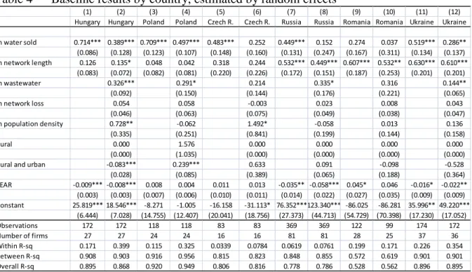
First, to see the robustness of the regression, we estimate it separately for some countries with enough observations. We report our results in Table 4.

Table 4 Baseline results by country, estimated by random effects

(1) (2) (3) (4) (5) (6) (7) (8) (9) (10) (11) (12)

Hungary Hungary Poland Poland Czech R. Czech R. Russia Russia Romania Romania Ukraine Ukraine ln water sold 0.714*** 0.389*** 0.709*** 0.497*** 0.483*** 0.252 0.449*** 0.152 0.274 0.037 0.519*** 0.286**

(0.086) (0.128) (0.123) (0.107) (0.148) (0.160) (0.131) (0.247) (0.167) (0.311) (0.134) (0.137) ln network length 0.126 0.135* 0.048 0.042 0.318 0.244 0.532*** 0.449*** 0.607*** 0.532** 0.630*** 0.610***

(0.083) (0.072) (0.082) (0.081) (0.220) (0.226) (0.172) (0.151) (0.187) (0.253) (0.201) (0.201)

ln wastewater 0.326*** 0.291* 0.214 0.335* 0.316 0.144**

(0.092) (0.150) (0.144) (0.176) (0.221) (0.065)

ln network loss 0.054 0.058 -0.003 0.023 0.008 0.043

(0.046) (0.063) (0.075) (0.049) (0.038) (0.047)

ln population density 0.728** -0.062 1.492* -0.058 0.013 0.136

(0.335) (0.251) (0.841) (0.199) (0.144) (0.158)

Rural 0.000 1.576 0.000 0.000 0.000 0.000

(0.000) (1.035) (0.000) (0.000) (0.000) (0.000)

Rural and urban -0.083*** 0.239*** 0.633 0.091 -0.098 -0.528

(0.028) (0.085) (0.389) (0.065) (0.188) (0.364)

YEAR -0.009*** -0.008*** 0.008 0.004 0.011 0.013 -0.035** -0.058*** 0.045* 0.046 -0.016* -0.022**

(0.003) (0.003) (0.007) (0.006) (0.010) (0.011) (0.014) (0.022) (0.027) (0.035) (0.009) (0.009) Constant 25.819*** 18.546*** -8.271 -1.005 -16.158 -31.113* 76.352***123.340*** -86.025 -86.281 35.996** 49.220***

(6.444) (7.028) (14.755) (12.407) (20.041) (18.756) (27.373) (44.713) (54.729) (70.398) (17.230) (17.052)

Observations 172 172 118 118 83 83 369 369 122 99 174 172

Number of firms 27 27 24 24 16 16 81 81 28 25 37 36

Within R-sq 0.171 0.399 0.115 0.325 0.0339 0.0784 0.0619 0.0761 0.199 0.171 0.226 0.354

Between R-sq 0.908 0.903 0.916 0.956 0.815 0.823 0.848 0.855 0.572 0.619 0.901 0.901

Overall R-sq 0.895 0.868 0.920 0.949 0.806 0.816 0.778 0.786 0.528 0.562 0.896 0.895

First, it is reassuring that the coefficients of outputs are similar across countries, suggesting that our cost function in (1) may characterize well the data at hand. The estimated coefficients consequently show that water quantity drives electricity consumption and wastewater quantity matters less. The sum of the two coefficients is significantly smaller than 1 for all countries, showing strongly increasing returns to scale. Network length is significant in Russia, Romania and Ukraine. The other variables, on the other hand, do not show strong patterns across countries, which may be a consequence of the relatively small sample size or the large extent of technological heterogeneity.

The next issue is to estimate the baseline equation for a pooled sample of firms in different countries. We show results separately for Visegrad countries (Czech Republic, Hungary, Poland, Slovakia), CEE countries and CIS countries in Table 5. The regression is estimated only for firms producing both water and wastewater, and includes a full set of country dummies.

22 Table 5 Pooled estimation

(1) (2) (3) (4) (5) (6) (7) (8)

V-4 V-4 CEE CEE CIS CIS all countries all countries

ln water sold 0.643*** 0.338*** 0.484*** 0.400*** 0.529*** 0.378*** 0.522*** 0.369***

(0.051) (0.034) (0.128) (0.140) (0.048) (0.066) (0.047) (0.061) ln network length 0.148*** 0.191*** 0.438*** 0.391*** 0.508*** 0.402*** 0.466*** 0.391***

(0.054) (0.060) (0.164) (0.144) (0.049) (0.030) (0.060) (0.049)

ln wastewater 0.271*** 0.101 0.119** 0.145***

(0.051) (0.085) (0.058) (0.045)

ln network loss 0.041*** 0.058** 0.110*** 0.083***

(0.009) (0.029) (0.029) (0.025)

ln population density 0.117 -0.038 -0.024 -0.035

(0.122) (0.065) (0.071) (0.046)

Rural 0.554 0.315 -0.429*** 0.049

(0.588) (0.252) (0.099) (0.262)

Rural and urban -0.082*** -0.098** -0.025 -0.032

(0.018) (0.048) (0.037) (0.035)

YEAR -0.005 -0.005 0.001 0.002 -0.029* -0.026** -0.018* -0.016*

(0.005) (0.005) (0.010) (0.008) (0.016) (0.013) (0.011) (0.009)

Observations 383 381 682 643 1002 992 1684 1635

Number of firms 71 70 180 173 203 202 383 375

Within R-sq 0.0618 0.212 0.00533 0.0133 0.0424 0.0590 0.0264 0.0403

Between R-sq 0.901 0.887 0.774 0.784 0.930 0.933 0.892 0.896

Overall R-sq 0.885 0.862 0.750 0.769 0.917 0.921 0.890 0.896

The table reinforces our earlier conclusions. First, coefficients of water and wastewater output are similar across countries. Increasing both by 10 percent ceteris paribus leads to about 5 percent increase in electricity consumption, showing very strong returns to scale. The effect of network length, and thus density, is significant in all country groups. This, however, is more important for CIS countries: while a 10 percent increase of the network (given water output) increases use by 1.9 percent in Visegrad countries, this increase is 4 percent in CIS countries.

This suggests that network operating costs and thus fixed costs are more important in these countries.

In these regressions network loss is significant, and its coefficient varies across country groups: it seems to be the most important for CIS countries, where 10 percent increase in network loss is associated with 1.1 percent larger electricity consumption. Interestingly, population density and the nature of service area have not been found to be related to energy efficiency. The time trend is significant for CIS countries suggesting about 3 percent increase in electricity efficiency per year.

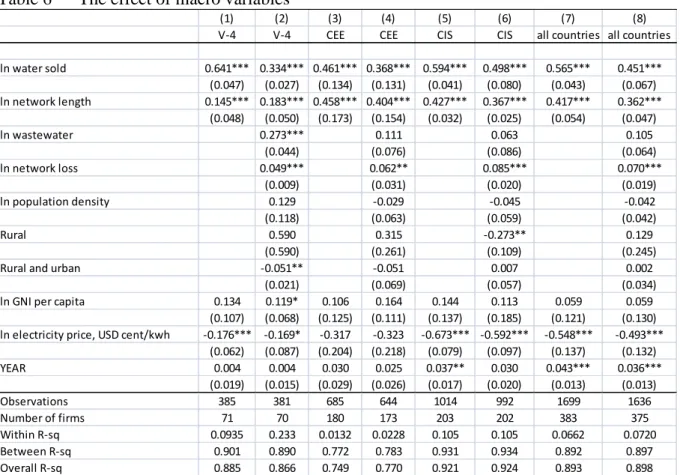
Next, we study how macro variables are related to electricity efficiency. For this, we include GNI per capita and electricity price to the regression. Note, that we also included country dummies to control for fixed characteristics of the countries, so identification comes from change in income and electricity prices. The results are reported in Table 6. The estimates show a very significant relationship between electricity price and energy efficiency:

23

increasing electricity prices by 10 percent leads to 4.9 percent decrease in electricity consumption given output. This effect is very strong in CIS countries, but also present to some extent in Visegrad countries: here a 10 percent increase in electricity price is associated with 1.7 percent increase in energy efficiency, suggesting that a lot of the efficiency improvement potential has already been utilized. These results point strongly to the importance of proper electricity prices in motivating firms to become more efficient. If one omits country dummies (unreported) the relationship between electricity prices and efficiency remains similar, but the regressions show a positive relationship between electricity use and GNI/capita.

Table 6 The effect of macro variables

(1) (2) (3) (4) (5) (6) (7) (8)

V-4 V-4 CEE CEE CIS CIS all countries all countries

ln water sold 0.641*** 0.334*** 0.461*** 0.368*** 0.594*** 0.498*** 0.565*** 0.451***

(0.047) (0.027) (0.134) (0.131) (0.041) (0.080) (0.043) (0.067) ln network length 0.145*** 0.183*** 0.458*** 0.404*** 0.427*** 0.367*** 0.417*** 0.362***

(0.048) (0.050) (0.173) (0.154) (0.032) (0.025) (0.054) (0.047)

ln wastewater 0.273*** 0.111 0.063 0.105

(0.044) (0.076) (0.086) (0.064)

ln network loss 0.049*** 0.062** 0.085*** 0.070***

(0.009) (0.031) (0.020) (0.019)

ln population density 0.129 -0.029 -0.045 -0.042

(0.118) (0.063) (0.059) (0.042)

Rural 0.590 0.315 -0.273** 0.129

(0.590) (0.261) (0.109) (0.245)

Rural and urban -0.051** -0.051 0.007 0.002

(0.021) (0.069) (0.057) (0.034)

ln GNI per capita 0.134 0.119* 0.106 0.164 0.144 0.113 0.059 0.059

(0.107) (0.068) (0.125) (0.111) (0.137) (0.185) (0.121) (0.130) ln electricity price, USD cent/kwh -0.176*** -0.169* -0.317 -0.323 -0.673*** -0.592*** -0.548*** -0.493***

(0.062) (0.087) (0.204) (0.218) (0.079) (0.097) (0.137) (0.132)

YEAR 0.004 0.004 0.030 0.025 0.037** 0.030 0.043*** 0.036***

(0.019) (0.015) (0.029) (0.026) (0.017) (0.020) (0.013) (0.013)

Observations 385 381 685 644 1014 992 1699 1636

Number of firms 71 70 180 173 203 202 383 375

Within R-sq 0.0935 0.233 0.0132 0.0228 0.105 0.105 0.0662 0.0720

Between R-sq 0.901 0.890 0.772 0.783 0.931 0.934 0.892 0.897

Overall R-sq 0.885 0.866 0.749 0.770 0.921 0.924 0.893 0.898

We also included three other variables in the regressions. First, we included a dummy whether the service area is hilly, i.e. whether the standard deviation in height is larger than 20 meters (as discussed in Chapter III.3). Second, we included a dummy whether the firm applies secondary treatment for wastewater. Third, we included the (ln) volume of water sold which is treated bulk. We assume that this requires less electricity than water distributed directly to consumers. Table 7 shows the results.