DETERMINANTS OF TOTAL FACTOR PRODUCTIVITY IN VISEGRAD GROUP
NUTS-2 REGIONS
Barbara DANSKA-BORSIAK
(Received: 10 August 2016; revision received: 3 March 2017;
accepted: 16 March 2017)
This article attempts to estimate the total factor productivity (TFP) for 35 NUTS-2 regions of the Visegrad Group countries and to identify its determinants. The TFP values are estimated on the basis of the Cobb-Douglas production function, with the assumption of regional differences in productivity. The parameters of the productivity function were analysed with panel data, using a fi xed effects model.
There are many economic variables that infl uence the TFP level. Some of them are highly cor- related, and therefore the factor analysis was applied to extract the common factors – the latent variables that capture the common variance among those observed variables that have similar pat- terns of responses. This statistical procedure uses an orthogonal transformation to convert a set of observations of possibly correlated variables into a set of values of linearly uncorrelated variables called principal components. Each component is interpreted using the contributions of variables to the respective component.
I estimated a dynamic panel data model describing TFP formation by regions. An attempt was made to incorporate the common factors among the model’s explanatory variables. One of them, representing the effects of research activity, proved to be signifi cant.
Keywords: Total Factor Productivity (TFP), Visegrad Group, regional analysis, dynamic panel data model, factor analysis
JEL classifi cation indices: C01, C23, E22, O33, O47
Barbara Danska-Borsiak, Chair of Spatial Econometrics, University of Łódź, Faculty of Econom- ics and Sociology. E-mail: danska@uni.lodz.pl
1. INTRODUCTION
Total factor productivity (TFP) growth can be used to assess changes in the effec- tiveness of the production process induced by technological progress. The change in efficiency is one of the determinants of economic growth.
Being a key factor in the improvement of social living standards, economic growth is of great interest to policy makers and researchers. One of the most pro- found recent studies was presented by Timmer et al. (2010), who had used data for the EU countries and the USA. One of their conclusions was that the differ- ences in labour productivity growth among the EU countries are mainly driven by the differences in their efficiency of using the inputs of basic production fac- tors. Other authors (e.g. Barro 1991; Miller – Upadhyay 2000) pointed out that many factors may affect output growth only through their effect on productivity.
Easterly – Levine (2001: 179) argued that “in searching for the secrets of long- run economic growth, a high priority should be placed on rigorously defining the term TFP, empirically dissecting TFP, and on identifying the policies and the institutions most conducive to TFP growth.” In the same paper they stated that over 90% of the differences in growth rates among nations are explained by TFP rather than by traditional factor accumulation. Moreover, regional disparities are larger and more persistent than cross-country differences, at least within the in- dustrialised countries (e.g. Magrini 2004).
The main objective of this paper is to identify the factors influencing the formation of TFP in the NUTS-2 regions of the Visegrad Group countries. The Visegrad Group, also known as the Visegrad Four or V4, was founded in 1991 in order to successfully accomplish social transformation and join in the European integration process. The members of the group are the Czechoslovak Republic (the Czech Republic and the Slovak Republic since 1993), Hungary, and Poland.
The participating countries cooperate mainly in the fields of culture, environ- mental protection, internal security, defence, science, and education. They were all members of the communist bloc for over 40 years. Central control, typical for the economies of this bloc, resulted in their technological backwardness and inefficiency. The Visegrad Group countries thus closely cooperated in efforts to- wards accession to the Euro-Atlantic structures. They had to overcome similar economic problems, especially ones related to improving productivity. Thus, it seems reasonable to analyse the common factors in TFP formation in the region of these countries and to determine the region-specific factors.
2. TOTAL FACTOR PRODUCTIVITY:
DETERMINANTS AND EMPIRICAL STUDIES REVIEW
TFP is interpreted as the volume of production per unit of a combination of fac- tors of production. As broadly understood, TFP, unlike productivities of particular production factors, is a synthetic measure of the efficiency of production process resulting from technical progress.
2.1. Determinants of TFP – literature review
Isaksson (2007: 2) orders the determinants of TFP into four groups:
– creation, transmission, and absorption of knowledge, – factor supply and efficient allocation,
– institutions, integration, invariants (geography), and policy, and – competition, social dimension, and environment.
For each group of determinants he discusses a list of related variables. Within the first group, Isaksson indicates research and development (R&D), some com- mon channels for the transfer of knowledge (e.g. trade, FDI), and requirements for the effective adoption of technology. Among the next group of determinants, the following factors are deemed important: human capital (e.g. education, health- care, and training), physical infrastructure (e.g. roads and electricity), physical capital, structural change (e.g. allocation of resources to the most productive sec- tors), and the financial system. Among institutions, a distinction is made between political (e.g. autocracy vs. democracy) and economic institutions, whereas in the case of integration, the focus is on trade. Geography and policy concentrate on the location of countries and their overall economic development such as per capita income levels and inflation. Within the last group, competition can be reflected by the effects of privatisation and the regulation of natural monopolies. What is primarily meant by the social dimension is income distribution and the wealth of an economy as well as, to some extent, social policy interventions. Considering environmental issues in the TFP framework as a new approach, Isaksson (2007:
73) argues that the environment can be seen as a production factor, as the deple- tion of natural resources (e.g. overuse of clean water) and the degradation of the environment (e.g. air pollution) can negatively influence welfare.
TFP determinants can also be viewed in either the long term or the medium term. According to the growth literature, the first group encompasses the factors called “deep determinants”, while the second group can be referred to as proxi- mate. Out of the four above-mentioned groups, the factors belonging to the last two are considered the deep determinants. They play an important role in TFP
formation because the medium-term policies influencing TFP (e.g. improving the allocation of resources) cannot be carried out effectively without good institu- tions. Identifying the deep determinants can help policy makers to improve their approaches to policy-making by, for example, producing a better understanding of the conditions under which some policies are more likely to work. Most of the deep determinants are persistent processes and are decided at the country level.
The above-mentioned factors influencing TFP growth lie on the supply side of the economy. However, the demand side determinants also matter, because demand pressures can trigger producers’ decisions with respect to, for example, technology adoption.
Hulten (2001: 40) noted that the TFP growth rate describes changes in the amount of output that can be produced by a given quantity of inputs. These changes result from technical innovations, organisational and institutional changes, shifts in societal attitudes, fluctuations in demand, or changes in factor shares. The fac- tors comprising TFP cannot be measured directly – only their aggregate effect is estimable, usually as a so-called “Solow residual”. According to Isaksson (2007:
1–4), the growth of TFP together with capital deepening influences growth in labour productivity and contributes to an increase in the welfare of people.
2.2. Empirical studies on TFP – a brief review
The majority of empirical studies on TFP and its determinants are conducted at the country level because of the availability of data. Scarpetta et al. (2002) carried out research into 10 OECD countries that have access to common technologies and are strongly linked by trade and investment. They found that stringent regula- tory settings in the product market and high hiring and firing costs negatively af- fect TFP. Theoretically, social policy affects income inequality, which in turn has a negative influence on productivity growth. According to Arjona et al. (2001) and Watson (2002), only those social expenditures that promote adjustment and labour market participation facilitate labour productivity growth. Other kinds of social expenditures may have negative or negligible effects. Recent literature suggests that environmental regulations have a positive impact on TFP and that they can lead to a faster rate of technological change (for an example see Isaksson 2007: 73–76).
Our empirical research deals with the NUTS-2 level, not the country level.
However, an attempt has been made to reflect the deep determinants in the model of regional TFP formation by including dummy variables for countries. Cornwall – Cornwall (2002) have decomposed productivity growth of 16 OECD econo- mies into the part caused by its changing structure and the part explained by
demand conditions. They conclude that strong aggregate demand leads to a wide- spread adoption of new technologies by stimulating investment and technological change.
Empirical studies on the Visegrad Group are also mostly related to the country level. Recent years have seen increasing research conducted at the NUTS-2 level.
However, according to our knowledge, there are no studies on the TFP formation at the NUTS-2 level of the V4 group.
Nežinský – Fifeková (2014) undertook a study on the sources of economic growth in the V4 countries during 2000–2013. They estimated the effect of TFP on growth in the broader context of examining the efficiency of transforming in- puts of capital and labour into output (measured as GDP), and alternative sources of growth, especially foreign direct investments. They found that TFP was a sig- nificant long-term pro-growth factor. Its influence was strongest in the Czech Republic and Slovakia. Some interesting findings come from decomposing the whole analysed period into three time spans. The highest growth of TFP, meas- ured as the average annual percentage change in constant prices, was observed in the years 2000–2003; the growth was only slightly lower during 2004–2007 and then dropped rapidly after 2008, which was interpreted as the effect of the economic crisis.
Another analysis of TFP in Visegrad countries is presented by Hloušek (2007), using quarterly data from 1996Q1 to 2006Q4. TFP growth was estimated by using the dual approach to growth accounting based on factor prices rather than quanti- ties. He argues that the primal (based on the Solow residual) and dual measures of the TFP growth rate should be the same. The labour-income share was esti- mated as a ratio of total labour cost to gross value added; it sums up to 1 with the capital-income share. The results showed that the highest average growth rate of TFP took place in Hungary and the Czech Republic, while Slovakia had the lowest TFP growth rate. The growth of TFP in terms of the growth of output was also calculated: in the case of the Czech Republic, TFP constitutes nearly 75%
of output growth, in Hungary it was about 50%, while in Poland and Slovakia it was 29% and 21%, respectively. Using quarterly data from 1995Q1 to 2004Q4, Hloušek applies the concept of growth accounting derived from the neoclassical production function. Arguing that the time series of capital are unavailable, he separates the part of output growth that represents the accumulation of capital and technology progress, treating it as the residual term, consisting of the contribution of both capital and technology progress. From time series of the growth rates, the amount of capital and/or technology progress is reconstructed in the form of an index. In 2004, this index takes the highest value for Poland and the lowest value for the Czech Republic. A growing tendency was observed during the whole pe- riod of analysis.
Golejewska (2013a, 2013b) covered the economies of the NUTS-2 regions of the Visegrad Group. The main focus of these analyses is either on competitive- ness and innovativeness, or on comparison of competitiveness and human capital intensity. She concluded that in the V4 NUTS-2 regions, innovations had a posi- tive and growing impact on regional competitiveness and that human capital has a positive impact on regional competitiveness. However, the results are of some interest in the context of the presented analysis because the positive effect of in- novation on labour productivity and TFP was confirmed in numerous analyses.
An econometric framework of the relation between productivity and innovation is presented in Vieira et al. (2011).
3. STATISTICAL DATA
I used panel data for the NUTS-2 regions of the Visegrad Group countries. There are 35 regions in the sample: eight from the Czech Republic, seven from Hun- gary; four from the Slovak Republic, and sixteen from Poland. The period under analysis covers the years 2000–2013.1
An important limitation often encountered in regional empirical analyses is the lack of certain data. In the context of our analysis, this problem specifically relates to regional measures of FDI and volume of trade, which could serve as channels for transferring knowledge between regions, and detailed information on social expenditures, which can influence labour productivity growth both positively and negatively. Another problem is that many of the TFP determinants were formulated at the national level. This is valid for all the deep determinants such as the quality of institutions, privatisation policy, regulatory schemes in the prod- uct market, or environmental regulations. As an attempt to introduce these fac- tors into our analysis, country dummy variables are included in the econometric model presented in Section 5.3.
The statistical data were taken from Eurostat. For the first step of analysis – the estimation of TFP – the following data (at constant prices) were needed:
GDP – gross domestic product in millions of euro L – labour input in thousands of employees
K – gross fixed capital formation in millions of euro
The analysed regions are highly diversified in terms of economic potential.2 As presented in Table 1, the ratio of quartile deviation to the median is over 30%
for GDP and gross fixed capital, and near 30% for employment. Moreover, this
1 The year 2013 was the last year for which data on all the necessary variables were available.
2 The summary statistics of the variables are presented in Table 2.
differentiation has increased over the analysed period and the largest increase oc- curred in the case of output.
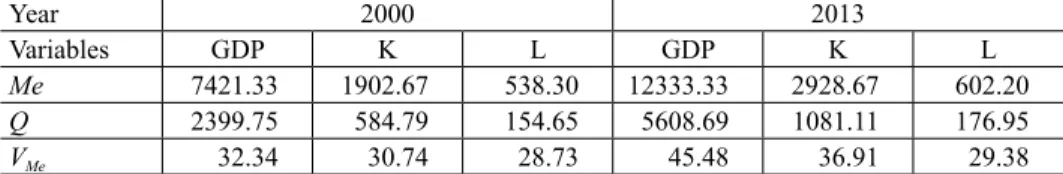
Figure 1 presents maps on which values of GDP, gross fixed capital, and number of employees are grouped into six categories: four quartiles plus two outlier categories at the low and high end of the distribution. It can be observed that in every case, there are no lower outliers, but most of the 35 regions fall into quartiles 1, 2, or 3. In most cases, the regions (including the capitals of the four countries) are characterised by the highest values of variables. The exception is Slovakia, where only the gross fixed capital value in 2013 takes the highest value of all NUTS-2 regions.
Another set of explanatory variables was necessary for the second step, for estimating an econometric model of TFP formation. It consists of a large number of variables, from which the so-called common factors were first extracted by means of the factor analysis method. The list of these variables is as follows:
edu02 – the percentage of employees with pre-primary, primary, and low- er secondary education (levels 0-2) in the total number of em- ployees (%)
edu56 – the percentage of employees with first and second stage of tertiary education (levels 5 and 6) in the total number of employees (%) patmi – number of patent applications to the EPO by priority year, per
million labour force
RDexp – total intramural R&D expenditure (GERD) as a percentage of GDP (%)
empl_ag – the percentage of employment in agriculture and fishing in total employment (%)
empl_ico – the percentage of employment in industry and construction in to- tal employment (%)
empl_tech – the percentage of employment in technology and knowledge-in- tensive sectors in total employment (%)
Table 1. Variation of the economic potential of the Visegrad Group NUTS-2 regions
Year 2000 2013
Variables GDP K L GDP K L
Me 7421.33 1902.67 538.30 12333.33 2928.67 602.20
Q 2399.75 584.79 154.65 5608.69 1081.11 176.95
VMe 32.34 30.74 28.73 45.48 36.91 29.38
Notes: The symbol Me denotes median, Q quartile deviation, and V quartile variation coefficient (in %).
Source: Author’s own calculations.
Figure 1. GDP, inputs of capital and labour in NUTS-2 regions
Notes: Territories of the four countries as well as regions including capital cities (darkest colour) are marked on the small map below the legend.
Values are classified as outliers if they are 1.5 times higher than the interquartile range (IQR). IQR is the differ- ence between the 75th percentile and the 25th percentile.
Source: Developed by the author.
Year 2000 Year 2013
GDP GDP
K K
L L
whour – average number of usual weekly hours of work in one’s main job (hours)
doct – number of physicians or doctors per 100,000 inhabitants
Apart from the common factors extracted from the variables listed above, the following variables, indicated in the literature cited in Section 2, were tested in the model:
U – unemployment rate (%)
CPI – consumer price index
dCZ, dHU, dPL, dSK – dummy variables indicating countries
The dummy variables have been treated as proxies of institutional and eco- nomic factors specific to each country. The summary statistics of these variables are presented in Table 2.
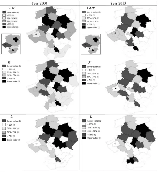
Table 2. Summary statistics for the variables used in the model
Variables Mean Std. Dev. Min Max Observa-
tions
GDP overall 13807.33 10666.42 4438.095 72390.58 N = 490
between 10336.02 5473.795 54500.18 n = 35
within 3117.913 1434.134 31697.73 T = 14
L overall 730.7462 400.1695 299.7 2479.5 N = 490
between 400.9872 315.8182 2146.627 n = 35
within 59.43219 402.0735 1063.619 T = 14
K overall 3080.278 2382.061 726.1376 16250.14 N = 490
between 2258.877 1038.964 12157.86 n = 35
within 839.3843 -617.4808 7443.473 T = 14
TFP overall 9.001979 1.517567 6.168093 15.36887 N = 490
between 1.236869 7.599023 12.66178 n = 35
within 0.9016675 5.834575 12.38968 T = 14
U overall 11.68909 6.020601 1.9 27.3 N = 490
between 4.733105 3.336364 20.16364 n = 35
within 3.79852 1.016364 21.42545 T = 14
CPI overall 1.00805 0.1107787 0.7527 1.297 N = 490
between 0.0135474 0.9743182 1.018909 n = 35
within 0.1099689 0.7430044 1.286904 T = 14
4. METHODOLOGY
I used factor analysis and dynamic panel data models. Factor analysis made it possible to extract the so-called “common factors” from 9 original variables de- termining the formation of TFP. Panel data models were used to estimate the influence of explanatory variables on TFP.
4.1. Factor analysis
The key concept of factor analysis3 is that multiple observed variables have similar patterns of responses because they are all associated with a latent variable. Thus, the basic idea of factor analysis is as follows: each observable, standardised input variable Zj is modelled as a linear combination of a number of unobserved vari- ables, the so-called (common) factors, common for the whole input set, and one unobserved factor specific for each variable. The common factors and the specific factors are uncorrelated with each other. This means that:
1 k ,
j jl l j j
l
Z w F b U
j= 1,2,...m, l = 1,2,...k,
where Fl is a l-th common factor, Uj is a j-th specific factor, the coefficients wjl and bj are called factor loadings in a j-th observable variable of common factor
3 A detailed and throughout description of the concept and method of factor analysis is given , e.g., at: http://documentation.statsoft.com/STATISTICAHelp.aspx?path=Factor/Indices/
Factor Analysis_HIndex
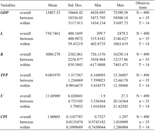
Table 2. continued
Variables Mean Std. Dev. Min Max Observa-
tions Factor_1 overall 1.01e-09 1 –1.314284 3.953619 N = 490
between 0.9798619 –1.088161 3.442386 n = 35
within 0.2547037 –1.763545 1.031639 T = 14
Factor_2 overall 1.36e-09 1 –2.089909 2.465256 N = 490
between 0.9419222 –1.567723 1.611634 n = 35
within 0.3686289 –1.489365 1.060683 T = 14
Factor_3 overall 1.13e-09 1 –3.309249 2.037808 N = 490
between 0.8665705 –1.775259 1.387614 n = 35
within 0.5182773 –1.635763 1.65158 1 T = 14
Fl, and of the j-th specific factor Uj, respectively. In order to identify common and specific factors, the factor loadings wjl and bj are estimated. They represent correlations between the j-th observed variable and the l-th common factor, and range from –1 to 1. Because the estimates obtained in the first step are not a unique solution, the mutually orthogonal axes – the main factors are rotated to fix axes in such a way that the corresponding loadings ensure sharper distinctions in the meanings of the factors. This happens because rotation means redefining factors, so that their loadings tend to be very high (–1 or 1) or very low (0), and high loadings provide the meaning and interpretation of factors.
4.2. Panel data models
Panel data combine two dimensions: the time dimension T and the cross-section dimension N, and thus provide multiple observations on each individual in the sample. One of the most valuable features of panel data is their theoretical ability to isolate the effects of specific actions, treatments, or policies.
A distinctive feature of models estimated from this kind of data is that con- stant-over-time and object-specific group effects are introduced. These group ef- fects capture unobservable, individual specific effects that are not included in the regression otherwise. Another distinctive property of panel data models is that their dynamic form requires specific methods of estimation because the meth- ods designed for static cases are not valid for dynamic models (see, e.g., Baltagi 2008: 147–148). A dynamic panel data model has the form:
(1)
where: x is a vector of explanatory variables, α0, γ, and β are parameters,
~ (0, 2)
it IID ε
ε σ and αi are the time invariant group effects, i = 1,…, N, t = 1,…, T.
An overview of the alternative methods of estimating the dynamic panel data models can be found in Baltagi (2008) and Hsiao (2003). One of the possible ap- proaches is based on the Generalised Method of Moments (GMM). In particular, this method allows for making alternative assumptions about the correlation be- tween the explanatory variables (all or some of the elements of vector xit of model 1) and the random term εit. The two most frequently-used methods of estimating dynamic panel data models are the first-differenced GMM (FDGMM) proposed by Arellano – Bond (1991) and the system GMM (SGMM) proposed by Blundell – Bond (1998).
FDGMM requires an assumption of non-autocorrelation of the error term εit in equation (1). In the first step, the group effects αi are removed by calculating first differences of (1). In the second step, the explanatory variables of the first-
0 , 1 T ( )
it i t it i it
y α γy x β α ε
differenced model are replaced with appropriate instruments and then the GMM is applied. The FDGMM estimators can be heavily biased when the lagged levels of the variables are only weakly correlated with subsequent first differences, so that the instruments available for the first differenced equations are weak. This situation may happen when the time dimension is short, when the autoregressive parameter approaches 1, or when the ratio of the variance of the group effects (αit) to the variance of the transient shocks (εit) is too large. In these cases, the system GMM (SGMM) estimator offers better results.
Basically, the SGMM concept consists of estimating a system of equations consisting of (1) and the first differences of (1). In other words, the first differ- ences and the levels of the same model are estimated concurrently. Regarding the first-differences equations, we apply the same procedure as in the case of the FDGMM. In the level equations, the predetermined and endogenous explanatory variables are also instrumented by appropriate instruments, which are valid as- suming that εit does not show an autocorrelation and that the initial conditions of the form: E(αi Δyi2) = 0 for i = 1,...,N are true.
5. EMPIRICAL RESULTS
One way of estimating TFP is using the Solow’s production model. Such an ap- proach is well-known in regional research and was adopted by, e.g., Dettori et al.
(2012) and Derbyshire et al. (2013).
5.1. Estimation of TFP values
The following relationship based on the Cobb-Douglas production function was used:
(2) where: Y is the gross domestic product (GDP) at constant prices in millions of euro, L is labour input (thousands of employees), K is gross fixed capital for- mation at constant prices (in millions of euro), Aegt>0 is TFP, g is the rate of Hicks technological progress, and α is the elasticity of Y with respect to K. The values of the variables are observed for the i-th region (i=1,…,35) in the year t (t = 1,…,14).
According to equation (2), the productivity Yit/Lit depends on the capital-labour ratio Kit/Lit and TFP, with TFP (equal to Aegt) being the same across all regions
ln it ln ln it ,
it it
Y K
L A gt α L
and years. This assumption seems difficult to accept, but the group effects in the panel data model are designed to control for unobserved time-invariant region characteristics. Ultimately, the model used in the first step of estimating regional TFP values took the form:
(3)
where αi is a time-invariant group effect specific to i-th region, capturing the interregional unobservable differences which may influence the region’s produc- tivity.
Equation (3) is a panel data fixed-effects model. It was estimated using the within-group estimator. The following equation presents satisfactory results:
(4)
The symbol âi denotes 35s different intercepts specific to the i-th region. The estimated rate of the Hicks technological progress is 3.4%, and the elasticity of labour productivity with respect to the capital-labour ratio is 0.29. In addition, all the variables are statistically significant at the 5% level and the fit of the model is satisfactory (R2 = 0,78).
Using the estimates of model (3), TFP values in the i-th region and in the year t were calculated using the formula:
(5) where the exponent in the denominator is an estimate of the parameter α in model (3).
The values of TFP, calculated as described above, differ between regions and time. Figure 2 shows the rate of medium-term change in TFP measure for each region. Figure 3 shows the values of TFP for each region in the years 2000 and 2013, which were the first and the last year of the sample, respectively. The me- dium-term change rate was calculated as:
Tn(iG 1) 100%, where
As Figure 2 shows, there are only six regions out of 35 in which, on average, the values of TFP declined during the analysed period. Among them, four of the 16 Polish NUTS-2 regions are mostly rural areas and located in the country’s east- ern part (the Lubuskie (PL43), Swietokrzyskie (PL33), Podkarpackie (PL32), and
ln it i ln it it,
it it
Y K
L α gt α L ε
ˆ ˆ
ln it i 0.03402 0.2947ln it .
it it
Y K
L α t L
0.2947
( / )
( / ) ,
it it
it
it it
Y L
TFP K L
1 2013 2000
.
G n
i TFP
TFP
Warminsko-mazurskie (PL62) voivodeships); the other two come from the seven Hungarian NUTS-2 regions (Dél-Alföld (HU33) and Dél-Dunántúl (HU23), lo- cated in the south of the country). The remaining 29 regions are characterised by a positive medium-term rate of change in TFP. The growth is highest in the Mazowieckie region in Poland (PL12) and equals 5.2%. The Polish capital city is located in this region, which definitely influences the region’s economy. In Figure 2, there are also three other regions marked with the black line. These are characterised by the highest medium-term change rate of TFP in a given country.
One of them is Közép-Magyarország (HU10), where the capital city is located and its TFP growth is much higher compared to other Hungarian regions. The non-capital city regions in the Czech Republic and Slovakia have the highest rate
Figure 2. Medium-term rate of change in TFP in the Visegrad Group NUTS-2 regions
Ͳ2 Ͳ1 0 1 2 3 4 5 6
SK04 SK03 SK02 SK01 PL63 PL62 PL61 PL52 PL51 PL43 PL42 PL41 PL34 PL33 PL32 PL31 PL22 PL21 PL12 PL11 HU33 HU32 HU31 HU23 HU22 HU21 HU10 CZ08 CZ07 CZ06 CZ05 CZ04 CZ03 CZ02 CZ01
of TFP growth. These countries’ NUTS-2 regions have a similar level of TFP growth rate, with only one region in Czech Republic having a slower, but still positive rate of growth.
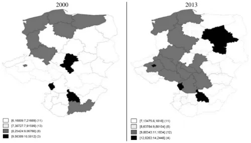
Figure 3 shows the estimated values of TFP in the 35 regions of the Visegrad Group. In the period from 2000 to 2013, the TFP level has increased. This is no- ticeable mainly in the Czech and Slovak regions, which belonged to the group of regions with the lowest productivity in 2000. Furthermore, a number of regions with a relatively higher TFP was larger in 2013, which are marked on the maps with darker colours.
5.2. Factor analysis – determinants of TFP
Following the estimation of TFP for each region, an attempt was made to identify which factors determine its formation. Section 2 presented a brief review of the literature concerning possible factors influencing TFP. Their number is high and they are interdependent to the extent that it is impossible to directly include all of them in the econometric model of TFP. For that reason, in the next step of the empirical research, the factor analysis method was applied to extract the so-called common factors without too much loss of information.
The characteristics used as the input variables are listed in Section 3. As a result of the principal components method, three common factors were distin-
Figure 3. TFP values in regions Source: Author’s calculation.
2000 2013
guished. Table 3 presents the variables associated with each factor, the factor’s eigenvalues, and the percentage of the overall variance explained by them.
The relationship of each variable to the underlying factor is expressed by the so-called factor loading, which can be interpreted like standardised regression coefficients. For the purpose of this analysis, those variables are chosen for which factor loadings exceed 0.65.
The eigenvalue is a measure of how much of the variance of the observed vari- ables is explained by a given factor. Factor_1 would explain as much variance as 3.1 of the four variables, and it captures 45.7% of the overall variance. This factor could be associated with the latent variable “effect of research activity”, as three out of the four variables indicate the effect of knowledge exploitation. The fourth variable clustered in Factor_1 is the number of physicians or doctors. This variable is considered as a proxy of government spending on health. In modern research, health and vital energy are often ranked among the components of hu- man capital. It can be argued that health has a direct effect on the productivity of workers, hence investments into healthcare can be regarded as good investments that increase the future productivity of individuals and the economy.
The next 22.7% of the overall variance is explained by Factor_2, which could be associated with the highest level of education and its use in industry and con- struction occupations. The third factor seems to represent the share of the agricul- tural sector in improving TFP.
These three factors, which jointly capture 80% of the overall variance in the initial set of ten variables, will thus be used in our analyses.
Table 3. Factor analysis results Variables Eigenvalue Percentage
of the overall variance
Cumulated
eigenvalue Cumulated percentage of the overall variance
Factor_1 patmi RDexp empl_tech doct
3.115137 45.72375 4.115137 45.72375
Factor_2 edu56
empl_ico 2.043491 22.70545 6.158628 68.4292
Factor_3 edu02
remplag 1.086716 12.07462 7.245344 80.50382
Source: Author’s calculation.
5.3. The econometric model of TFP
In order to identify the causes of interregional differences in TFP growth rates, growth models are generally used. Here, a dynamic panel data model is applied.
The model was estimated using the yearly data for the 35 NUTS-2 regions of the Visegrad Group from 2000 to 2013. Different explanatory variable sets were tested, as were different assumptions about the endogeneity of explanatory varia- bles, and two alternative estimation methods, namely FDGMM and SGMM were adopted. The estimation results of the final version are presented in Table 4. The model was estimated by SGMM with the variables Factor_1 and CPI, treated as endogenous.
Table 4. Estimation results of the TFP model Coeff. Robust std.
error t-stat p-value Hypotheses testing
TFPt-1 0.8097 0.036 22.50 0.000 Wald test:
chi2(5) = 606.66, p-value = 0.0000
Arrelano-Bond test:
m1 = –4.3947, p-value = 0.0000 m2 = 0.85498, p-value = 0.3926
Factor_1 0.1341 0.056 2.38 0.017
CPI –1.3732 0.4363 –3.15 0.002
d2008 0.6473 0.167 3.88 0.000
d2010 0.3592 0.101 3.56 0.000
_cons 3.1942 0.552 5.79 0.000
Notes: The Arellano-Bond test verifies the quality of the FDGMM or SGMM estimates.4 The occurrence of first-order autocorrelation is expected because if εit are independent, then its first differences are correlated of order 1. If the model has an autocorrelation of an order higher than 1 (as in H1), this would mean that the moment conditions are not true and that the instruments used in GMM-based estimation are not valid (Baltagi 2008:153).
Source: Author’s calculation.
The results shown in Table 4 indicate that TFP formation is highly persistent.
The lagged level of TFP strongly affects the current value (parameter estimate 0.8097). Among the three factors separated by means of the principal components method, only Factor 1 is significant in the model. Factor 1 is associated with the field of R&D and accessibility of medical care. The impact is not very strong, but it is positive and significant. It can be interpreted as implying that in order to increase TFP in a region, the most effective way is to direct additional outlays to R&D and to create jobs in technology and knowledge-intensive sectors. The
4 The alternative is the Sargan test. I use only the Arrelano-Bond test because I calculate the robust variance estimators. In that case, the empirical distribution of the Sargan test statistics is not known.
greater number of patent applications seems to be a result of these outlays. As good accessibility to medical care (approximated by the number of physicians or doctors) also contributes to TFP growth through Factor_1, increases in spending on healthcare may be another tool for enhancing TFP.
Two time dummies, d2008 and d2010, have also been included in the explanatory variable set. In both years, 2008 and 2010, the level of productivity was on aver- age higher than in other years. The year 2008 was the first year of the world eco- nomic crisis, but the economies of the Visegrad Group were outside the euro zone (with the exception of Slovakia, which, however, adopted the euro only in 2009).
For that reason, and also because of the relatively lower level of development of financial markets in these countries, the effects of the global financial crisis were weakened and delayed.
The consumer price index (CPI) is an additional variable in the model. It is included in the set of explanatory variables in order to measure the effects of inflation on economic efficiency (e.g. Miller – Upadhyay 2000).
I wanted to include some other variables indicated in the literature. However, most of the cited studies, as already mentioned above, deal only at country levels.
At the regional levels, some variables such as the volume of trade and the effects of privatisation are unavailable. Therefore, only the unemployment rate and the dummy variables were tested. The unemployment rate proved to be insignificant, possibly because it was too closely correlated with CPI. The dummy variables indicating countries were tested as proxies of institutional and economic factors specific to each country. In other words, our aim was to find out whether there are any country-level instruments that influence regional TFP. The dummies proved to be insignificant, which means either that there are no such influences, or that such an influence may be present, but its strength and direction may be similar for all analysed countries.
6. SUMMARY AND CONCLUSIONS
TFP is a variable which accounts for effects in total output growth relative to the growth in inputs, that is, labour and capital. This variable, which cannot be measured directly, was estimated for the NUTS-2 regions of the Visegrad Group.
The medium-term growth rate is greater than one in the vast majority of them.
This increase is especially noticeable in the Czech and Slovak regions, and in the Mazowieckie region, where Poland’s capital city is located.
By using the factor analysis method, common factors were extracted from nine observed variables, which were regarded as potential determinants of TFP. The one that proved to be statistically significant in the dynamic panel data model of
TFP formation was the factor associated mainly with the latent variable, “effect of research activity”. This factor captures 45.7% of the overall variance and also includes an indicator of health and vital energy. TFP formation is highly persist- ent. In the estimated model, the lagged level of TFP strongly affects the current value (parameter estimate 0.8097). The time series data used in the analysis is from 2000 to 2013. This period covers the year of the Visegrad countries acces- sion to the European Union (2004) and the year 2008, in which economic crisis took place. Yearly dummy variables were incorporated in the model to account for these circumstances, but they did not indicate any negative effect of the crisis on TFP. If such an impact occurred, it might have been captured by the variable representing inflation.
REFERENCES
Arellano, M. – Bond, S. (1991): Some Tests of Specifi cation for Panel Data: Monte Carlo Evidence and an Application to Employment Equations. Review of Economic Studies 58(2): 277–297.
Arjona, R. – Ladaique, M. – Pearson, M. (2001): Growth, Inequality and Social Protection. OECD Labour Market and Social Policy Occasional Papers, No. 51, Paris.
Baltagi, B. H. (2008): Econometric Analysis of Panel Data, 4th ed. Chichester: Wiley & Sons.
Barro, R. (1991): Economic Growth in a Cross Section of Countries. The Quarterly Journal of Economics, 106(2): 407–443.
Blundell, R. – Bond, S. (1998): Initial Conditions and Moment Restrictions in Dynamic Panel Data Models. Journal of Econometrics, 87(1): 115–143.
Cornwall, J. – Cornwall, W. (2002): A Demand and Supply Analysis of Productivity Growth. Struc- tural Change and Economic Dynamics, 13(2): 203–229. Available from: https://www.research- gate.net/publication/223374377_A_Demand_and_Supply_Analysis_of_Productivity_Growth, [accessed January 29, 2016].
Derbyshire, J. – Gardiner, B. – Waights, S. (2013): Estimating the Capital Stock for the NUTS2 Regions of the EU27. Applied Economics, 45(9): 1133–1149.
Dettori, B. – Marrocu, E. – Paci, R. (2012): Total Factor Productivity, Intangible Assets and Spatial Dependence in the European Regions. Regional Studies, 46(10): 1401–1416.
Easterly, W. – Levine, R. (2001): It’s Not Factor Accumulation: Stylized Facts and Growth Models.
The World Bank Economic Review, 15(2): 177–219.
Golejewska, A. (2013a): Human Capital and Regional Growth Perspective. Barometr Regionalny, 11(1): 7–17.
Golejewska, A. (2013b): Competitiveness, Innovation and Regional Development. The Case of the Visegrad Group Countries. Gospodarka Narodowa, 7–8: 87–112.
Hloušek, M. (2005): Growth Accounting – Application for Visegrad States. Available from: http://
econ.muni.cz/~hlousek/papers/growth.pdf [accessed December 29, 2016]
Hloušek, M. (2007): Growth Accounting for Visegrad States: Dual Approach. Working Paper, No.17/2007, Research Centre for Competitiveness of Czech Economy. Available from: http://
is.muni.cz/do/1456/soubory/oddeleni/centrum/papers/wp2007-17.pdf [accessed December 29, 2016]
Hsiao, C. (2003): Analysis of Panel Data. 2nd ed., Cambridge: Cambridge University Press.
Hulten, C. R (2001): Total Factor Productivity. A Short Biography. http://www.nber.org/chapters/
c10122.pdf [accessed January 29, 2016]
Isaksson, A. (2007): Determinants of Total Factor Productivity: A Literature Review. UNIDO, Re- search and Statistics Branch, Staff Working Paper, No. 02/2007.
Kisiała, W. – Bajerski, A. – Stępiński, B. (2017): Equalising or Polarising: The Centre-Periphery Model and Absorption of EU Funds under Regional Operational Programmes in Poland. Acta Oeconomica, 67(3): 413–434.
Magrini, S. (2004): Regional (Di)convergence. In: Henderson, V. – Thisse, J. F. (eds): Handbook of Regional and Urban Economics: Cities and Geography. Amsterdam: Elsevier, pp. 2741–2796.
Miller, S. – Upadhyay, M. (2000): The Effects of Openness, Trade Orientation, and Human Capital on Total Factor Productivity. Journal of Development Economics, 63(2): 399–423.
Nežinský, E. – Fifeková, E. (2014): The V4: A Decade after the EU Entry. Entrepreneurial Business and Economics Review, 2(2): 31–46.
Privatization and Regulation: Effi ciency and Equity Issues in Developing Countries. Papers from Meeting of Experts Hold by United Nations Department of Economic and Social Affairs. New York, 16–18 February 1999. Available from: http://unpan1.un.org/intradoc/groups/public/
documents /un/unpan000152.pdf , [accessed January 29, 2016]
Scarpetta, S. – Hemmings, P. – Tressel, T. – Woo, J. (2002): The Role of Policy and Institutions for Productivity and Firm Dynamics: Evidence from Micro and Industry Data. OECD Economics Department, Working Papers, No. 329, Paris.
Timmer, M. P. – Inklaar, R. – O’Mahony, M. – van Ark, B. (2010): Economic Growth in Europe.
New York: Cambridge University Press.
Vieira, E. – Neirad, I. – Vázquez, E. (2011): Productivity and Innovation Economy: Comparative Analysis of European NUTS-2, 1995–2004. Regional Studies, 45(9): 1269–1286.
Watson, W. (2002): Social Policy and Productivity: Anybody Here See Any Levers? The Review of Economic Performance and Social Progress, 2: 307–321.