Qualitative properties of discrete nonlinear parabolic operators

(will be inserted by the editor)

Qualitative properties of discrete nonlinear parabolic operators

R´obert Horv´ath · Istv´an Farag´o · J´anos Kar´atson

Received: date / Accepted: date

Abstract This paper is devoted to the qualitative properties of discretized parabo- lic operators, such as nonnegativity and nonpositivity preservation, maximum/mi- nimum principles and maximum norm contractivity. In the linear case, earlier papers of the authors [5, 6] have established the connections between the above qualitative properties and have given sufficient conditions for their validity. The present paper extends the above results to nonlinear discretized parabolic oper- ators, also motivated by the authors’ recent paper [8], which has given related results on the continuous PDE level. A systematic study is presented, ranging from general discrete mesh operators to proper finite element applications.

1 Introduction and preliminaries

The qualitative properties of the continuous and discrete solutions of partial dif- ferential equations are under intensive research nowadays. Namely, beyond the convergence of a numerical method, it is also important to preserve the character- istic qualitative properties of the modeled phenomenon to the numerical solution.

This guarantees that the numerical scheme actually used on computers is reliable and efficient. The preservation of the properties can be achieved by a deep analy- sis of the schemes and it is generally guaranteed with proper assumptions for the

R´obert Horv´ath

Department of Analysis at Budapest University of Technology and Economics and NUM-NET MTA-ELTE Research Group, Egry J. u. 1, H-1111, Budapest, Hungary

E-mail: rhorvath@math.bme.hu Istv´an Farag´o

Department of Differential Equations at Budapest University of Technology and Economics, Department of Applied Analysis and Computational Mathematics at E¨otv¨os Lor´and Univer- sity, and NUM-NET MTA-ELTE Research Group, Egry J. u. 1, H-1111, Budapest, Hungary E-mail: faragois@cs.elte.hu

J´anos Kar´atson

Department of Applied Analysis and Computational Mathematics at E¨otv¨os Lor´and Uni- versity, Department of Analysis at Budapest University of Technology and Economics and NUM-NET MTA-ELTE Research Group, P´azm´any P. stny. 1/c, H-1111, Budapest, Hungary E-mail: karatson@cs.elte.hu

spatial discretization and the time-step. For linear parabolic problems the most extensively studied properties are the different maximum and minimum principles, the nonnegativity and nonpositivity preservation and the maximum norm contrac- tivity. Such results can be found in the works [1, 5, 7, 15, 16, 20–22, 24–27] and in the references therein. Not only the preservation of the qualitative properties are important themselves but also their relations. These relations were revealed in an organized framework using discrete mesh operators for linear discrete parabolic problems in an earlier paper of the authors [6].

In the recent decades the interest has turned to the more complicated case of various nonlinear problems in this context, see e.g. [9, 12–14, 19, 23, 28] where sufficient conditions are given for the qualitative properties, usually related to maximum/minimum principles. However, a study of the relations between such properties has not been carried out yet. Our goal is to give a systematic study on this topic for proper classes of nonlinear problems. Besides the mentioned linear case [5, 6], we are motivated by the corresponding background on the continuous PDE level, on which we have derived similar results for certain nonlinear parabolic operators in [3, 8].

Let us consider the parabolic operator N[u]≡∂u

∂t −div K(x, t,∇u)

+q(x, t, u) (1)

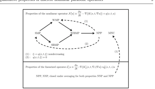
in the cylinder Ω×(0, T), where Ω is a bounded domain in R^d andT > 0 is a fixed number. The coefficientsK:Ω×(0, T)×R^d→R^d andq:Ω×(0, T)×R^→R are given sufficiently smooth functions. We also suppose thatK(x, t,0) = 0 and q(x, t,0) = 0. These conditions are not too restrictive, since the functions q and K generally describe some reaction process and flux quantity, respectively, which vanish in the absence of the given quantity. In [8], we have investigated the qual- itative properties of the operator (1) on the continuous level and revealed the implications between its properties. For different versions of minimum and max- imum principles (SMP, SBMP, WMP, WBMP), nonnegativity and nonpositivity preservation (NNP, NPP) and maximum norm contractivity (MNC), we have ob- tained the conditions summarized in Figure 1. We note that we have simplified the original figure to the case of Dirichlet boundary conditions, and a similar figure applies to minimum principles and nonnegativity preservation.

The goal of this paper is to derive the discrete versions of the above implications and other statements of our previous paper [8]. Thereby we also properly extend our earlier study on the linear parabolic case [5, 6], where a diagram analogous to Figure 1 has been given. We introduce general discrete mesh operators (DMOs), we define their qualitative properties, we characterize the relations between them and give sufficient conditions for the validity of these properties. Then we adapt this study to two-level mesh operators, and finally we apply the results to establish the preservation of the qualitative properties for proper finite element applications.

2 Nonlinear discrete parabolic mesh operators and the relations between their qualitative properties

LetΩbe again a bounded domain inR^d(d= 1,2, . . .) with the usual notation∂Ω for its boundary. The space mesh is described by the sets

Fig. 1 Connections between the qualitative properties of the nonlinear parabolic operator(1).

P ={x1, x2, . . . , x_N}andP_∂ ={x_N+1, x_N+2, . . . , x_N+N∂},

consisting of distinct points ofΩand∂Ω, respectively. We define ¯N=N+N_∂ and P¯= P∪P∂. LetT be again a positive number and ∆ta positive time-step such thatT =∆tnT for some positive integernT. For the time mesh we introduce the setR ={t∈R^|t=tn :=n∆t, n= 0,1, . . . , n_T}. For anyt∈R we introduce the notations

Rt:={τ∈R|0< τ < t}, Rt¯:={τ∈R|0< τ≤t}, R⁰t¯:={τ ∈R|0≤τ≤t}

and the sets

Qt=P×Rt, _Q¯_t= ¯P×R⁰_¯t, Q¯t=P×R¯t, Γt= (P_∂×R⁰_¯t)∪(P× {0}). Definition 1 A mapping from the space of real-valued functions defined on ¯Q_T to the space of real-valued functions defined onQT is called adiscrete mesh operator (DMO).

Thus, a DMO assigns mesh functions to mesh functions. The domain of a DMO D, that is the space of real-valued functions defined on ¯Q_T, is denoted by dom(D).

We define the qualitative properties of DMOs in an analogous way as they were defined for the nonlinear partial differential operator (1) in [8]. Inequalities are understood pointwise on the whole domain of the given mesh function.

Definition 2 A DMOD satisfies

(a) the discrete nonnegativity preservation (DNNP)property if:

v∈dom(D), t∈RT, D[v]|Qt¯≥0, v|Γ_t≥0, ⇒ v|Q¯t≥0;

(b) the discrete nonpositivity preservation (DNPP)property if:

v∈dom(D), t∈RT, D[v]|Qt¯≤0, v|Γ_t≤0, ⇒ v|Q¯t≤0;

(c) thediscrete weak boundary maximum principle (DWBMP) and the discrete strong boundary maximum principle (DSBMP), respectively, if for all t∈R_T andv∈ dom(D) withD[v]|_Q¯t≤0:

maxv|Q¯t ≤ (

max{0,maxv|_Γt} (DWBMP), maxv|Γ_t (DSBMP)

(DSBMP means that vattains its maximum on the parabolic boundary, and DWBMP means the same only for a nonnegative maximum);

(d) the discrete weak boundary minimum principle (DWBmP) and the discrete strong boundary minimum principle (DSBmP), respectively, if for all t ∈ R_T and v∈ dom(D) withD[v]|_Q¯t≥0:

minv|Q¯t ≥ (

min{0,minv|_Γt} (DWBmP), minv|Γ_t (DSBmP)

(DSBmP means that v attains its minimum on the parabolic boundary, and DWBmP means the same only for a nonpositive minimum);

(e) thediscrete weak maximum principle (DWMP) and the discrete strong maximum principle (DSMP), respectively, if for allt∈R_T andv∈dom(D):

maxv|Q¯t ≤







t·max{0,sup

Q¯t

D[v]}+ max{0,maxv|Γt} (DWMP), t·max{0,sup

Q¯t

D[v]}+ maxv|Γ_t (DSMP);

(DWMP and DSMP complete the bound in DWBMP and DSBMP, respec- tively, with a term includingD[v] when the latter has no prescribed sign);

(f) thediscrete weak minimum principle (DWmP) and the discrete strong minimum principle (DSmP), respectively, if for allt∈RT andv∈dom(D):

minv|Q¯_t≥







t·min{0,inf

Qt¯

D[v]}+ min{0,minv|_Γt} (DWmP), t·min{0,inf

Qt¯

D[v]}+ minv|Γ_t (DSmP);

(DWmP and DSmP complete the bound in DWBmP and DSBmP, respectively, with a term includingD[v] when the latter has no prescribed sign);

(g) the discrete maximum norm contractivity (DMNC) property if for anyt ∈ RT

and any two functionsv1, v2∈dom(D) such that D[v1] =D[v2] inQ¯t, v1|_P∂×R⁰

¯t =v2|_P∂×R⁰

t¯, the relation

max_x∈P¯|v1(x, t)−v2(x, t)| ≤max

x∈P^¯

|v1(x,0)−v2(x,0)| is valid.

Remark 1 (i) The above qualitative properties are formulated for mesh operators similarly to the linear case [6]. The analogous properties for corresponding systems of equations can be formulated in an obvious way. For example, the DNNP simply expresses that nonnegative data yield a nonnegative solution.

(ii) We have defined the maximum and minimum principles separately. It can be checked easily that if a DMODpossesses the propertyD[−v] =−D[v] (e.g. if Dis linear) for allv∈dom(D) then the maximum principles are equivalent to the corresponding minimum principles and the DNPP is equivalent to the DNNP.

We start with some straightforward relations between the above properties.

Proposition 1 For a DMO, the discrete strong maximum principles DSMP and DS- BMP imply the discrete weak maximum principles DWMP, DWBMP, respectively. The discrete maximum principles DSMP and DWMP imply the discrete boundary max- imum principles DSBMP and DWBMP, respectively. Similar statements are true for the minimum principles. If the operator satisfies one of the maximum (resp. minimum) principles then it also preserves the nonpositivity (resp. nonnegativity).

Proof These follow directly from the above definitions.

Now we investigate the implications in the opposite direction, that is we for- mulate conditions under which the DNPP implies the maximum principles. To this end, we introduce two special grid functions, the constant one 11 : ¯Q_T →R and the “functiont”tt: ¯Q_T →R, respectively:

11(x, t) := 1 for all (x, t)∈_Q¯_{T, tt}(x, t) :=t for all (x, t)∈_Q¯_T. The restrictions of these functions toQ_T will be denoted in the same way.

Theorem 1 Let a DMO D possess the following property: for all functions v ∈ dom(D)and for all nonnegative numbersαandβ, the relation

D[v−αtt−β11]≤D[v]−α11 (∀α≥0, β≥0) (2) is satisfied. Then the DNPP implies the DWMP and the DNNP implies the DWmP.

Proof Assume that the DMO D possesses the DNPP. Let v be a fixed function from dom(D) and lett∈RT be a fixed value. Let

M1:= max{0,sup

Q¯t

D[v]}, M2:= max{0,maxv|Γ_t}.

For the DWMP to hold, we must prove thatv(x, τ)≤M1t+M2(∀(x, τ)∈_Q¯_t).Let us define the new grid function ˜v=v−M1tt−M211.Then, based on the assumption of the theorem, we have

D[˜v] =D[v−M1tt−M211]≤D[v]−M111, which relation shows thatD[˜v]≤0 onQ¯t. Moreover

˜

v=v−M1tt−M211≤v−M211≤0

onΓt. The discrete nonpositivity preservation property (DNPP) implies that ˜v≤0 inQ¯t, thus also in ¯Qt, i.e.v≤M1tt+M2≤M1t+M2in ¯Qtas required.

The other implication regarding the minimum principle can be proven simi- larly. The valuesM₁ andM₂ must be defined with minimums and infimums, and condition (2) should be applied with the functionv:=v−M1tt−M211 and with

the parametersα=−M1andβ=−M2.

Theorem 2 Let a DMO D possess the following property: for all functions v ∈ dom(D)and for all nonnegative numberαand real numberβ, the relation

D[v−αtt−β11]≤D[v]−α11 (∀α≥0, β∈R) (3) is satisfied. Then the DNPP implies the DSMP and the DNNP implies the DSmP.

Proof The proof for DSMP is similar to the proof of Theorem 1, because the condition of the theorem guarantees the given estimation independently of the sign of β. To complete the proof we only need to redefine the parameter M2 as M2:= maxv|Γ_t. The case of DSmP can be obtained similarly.

Remark 2 Note that the conditions of Theorems 1–2 are generalizations of the conditions obtained for linear DMOs in [6]: D[11]≥0 (resp.D[11] = 0) andD[tt]≥ 1. This follows simply fromD[v−αtt−β11] =D[v]−αD[tt]−βD[11]≤D[v]−α11.

Now we consider the implication of the DMNC property. Similarly to the con- tinuous case in [8], we cannot deduce the DMNC of D directly from the DNNP and DNPP properties ofD. Instead, we must require the same properties for some linearized version of the operatorD, the so-calleddivided differencemesh operator, which is generally used to approximate derivatives.

Theorem 3 Let us suppose that the DMOD satisfies the following assumptions:

i) D[v−β11] ≤ D[v] is satisfied for all nonnegative values β and for all functions v∈dom(D);

ii) for all fixed functions w,¯ w˜ ∈ dom(D), there exists a DMO Lw,_¯w˜ that possesses both the DNNP and the DNPP properties, moreover, applying this operator to the function w¯−w, we obtain˜

Lw,_¯w˜[ ¯w−w˜] =D[ ¯w]−D[ ˜w]. Then the DMOD possesses the DMNC property.

Proof Let us suppose thatv1andv2are two arbitrary functions from dom(D) with the properties

D[v1] =D[v2] inQ¯t, v1|_P∂×R⁰

t¯=v2|_P∂×R⁰

¯t, (4)

wheret∈R_T is a fixed number. With the notationζ:= max

x∈P^¯|v1(x,0)−v2(x,0)|(ζ is a nonnegative number) we have to prove that

max

x∈P^¯

|v1(x, t)−v2(x, t)| ≤ζ. (5) Let us consider the function w⁻ = v₁−v₂−ζ11. This function is nonpositive on Γt. According to assumption ii), there exists a DMO Lv1,v2+ζ11, such that L_v1,v2+ζ11[v1−v2−ζ11] =D[v1]−D[v2+ζ11]≤D[v1]−D[v2] = 0. Here we applied assumption i) (with the choices v=v2+ζ11 andβ=ζ) and condition (4). Thus L_v1,v2+ζ11[w⁻]≤0. BecauseL_v1,v2+ζ11is nonpositivity preserving, this implies that w⁻≤0 onQ¯t(thus also on ¯Qt), that is

max

x∈P^¯

{v1(x, t)−v2(x, t)} ≤ζ. (6)

Similarly, let us consider the functionw⁺=v1−v2+ζ11. This function is nonneg- ative onΓt. According to assumptionii), there exists a DMOL_v1,v2−ζ11, such that L_v1,v2−ζ11[v1−v2+ζ11] =D[v1]−D[v2−ζ11]≥D[v1]−D[v2] = 0. Here we applied assumptioni) (withv=v₂andβ=ζ) and condition (4). ThusL_v1,v2−ζ11[w⁺]≥0.

Because Lv1,v2−ζ11 is nonnegativity preserving, this implies that w⁺ ≥ 0 on Q¯t

(thus also on ¯Qt), that is max_x∈P¯{v2(x, t)−v1(x, t)} ≤ζ.This estimate together

with (6) shows the required estimate (5).

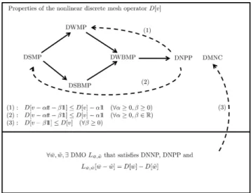
The implications proven in this section are summarized in Figure 2. For the discrete minimum principles and the DNNP the figure would be similar.

Fig. 2 Connections between the qualitative properties of a discrete nonlinear mesh operator.

In the next section, we formulate the above results and conditions for a special type of DMOs: for the so-called two-level DMOs.

3 Two-level DMOs and the relations between their qualitative properties For the sake of simplicity, we denote the value of a mesh functionv at the point (xi, tn) byv_iⁿ. Moreover, we introduce the column vectors

vⁿ= [vⁿ₁, . . . , vⁿN¯]^T, v₀ⁿ= [v₁ⁿ, . . . , vⁿ_N]^T, vⁿ_∂ = [v_Nⁿ₊₁, . . . , vNⁿ¯]^T.

In many numerical solution methods of parabolic partial differential equations, such as finite difference and finite element methods, DMOs appear in the following special form:

(D[v])ⁿi = (X₁^(vn)vⁿ−X^(v

n−1)

2 vⁿ⁻¹)i, i= 1, . . . , N, n= 1, . . . , n_T, (7) where X^(v

n) 1 , X^(v

n−1)

2 ∈R^N×N¯ are given matrices. Here the superscripts indicate that the matrices may depend on the vectorsvⁿ andvⁿ⁻¹, that is on the values of

the mesh functionvat the time levelstnandtn−1, respectively. These matrices may depend also on the indexnof the time level and on the time-step∆t, although for the sake of simplicity we do not indicate this dependence in the notation. Because in the computation of (D[v])ⁿ_i only thenth and (n−1)th time levels are involved, an operator in the form (7) is called atwo-level discrete mesh operator (DMO2). To shorten the writing of the formulas, we introduce the formal notation

J(w1, w2) :=X₁^(w1)w1−X₂^(w2)w2 (w1, w2∈R

N¯

).

Then (D[v])ⁿ=J(vⁿ, vⁿ⁻¹). Our goal is to formulate the conditions of the the- orems in the previous section to DMO2s. Let us introduce the column vector e := [1, . . . ,1]^T ∈ R^N¯.The N-element and the ( ¯N−N)-element versions of this vector will be denoted bye0 ande_∂, respectively.

Theorem 4 Condition (2)can be guaranteed for the DMO2 (7)by imposing the fol- lowing assumption on the matricesX₁^(.)andX₂^(.):

(W) J(w1−ae, w2−be)≤J(w1, w2)−^a−b_∆t e0for allw1, w2∈R^N¯ and for all nonnegative values a≥b≥0.

Proof It can be seen easily that condition (2) is equivalent with the condition J(vⁿ−αn∆te−βe, vⁿ⁻¹−α(n−1)∆te−βe)≤J(vⁿ, vⁿ⁻¹)−αe0 (8) (∀v ∈ dom(D), n ∈ {1, . . . , n_T}, α ≥ 0, β ≥ 0) for DMO2s. Thus, let v be an arbitrary fixed mesh function from dom(D),n∈ {1, . . . , n_T}a fixed number, and α≥0, β ≥0 two fixed nonnegative numbers. Assumption (W) with the choices a=αn∆t+β,b=α(n−1)∆t+β,w1=vⁿandw2=vⁿ⁻¹ results in the required

condition (8) directly.

Condition (3) can be guaranteed with a stricter condition, where the sign of the parametersaandbis not fixed unlike in condition (W).

Theorem 5 Condition (3)can be guaranteed for the DMO2 (7)by imposing the fol- lowing assumption on the matricesX₁^(.)andX₂^(.):

(S) J(w1−ae, w2−be)≤J(w1, w2)−^a−b_∆t e0 for all w1, w2∈R^N¯ and for all values a≥b.

Proof We have to guarantee condition (8) again but now with arbitrary real values β. The validity of the condition can be proven in a similar way as for the previous

theorem.

The letters W andS in the notations of the above assumptions indicate that these assumptions guarantee the validity of the weak and strong maximum prin- ciples, respectively. This is shown by the next theorem.

Theorem 6 If a DMO2 possesses the DNPP property and fulfills condition(W), then it possesses all the weak maximum principles DWMP and DWBMP. If a DMO2 pos- sesses the DNPP property and fulfills condition(S), then it possesses all the maximum principles DWMP, DSMP, DWBMP and DSBMP.

Similarly, if a DMO2 possesses the DNNP property and fulfills condition(W), then it possesses all the weak minimum principles DWmP and DWBmP. If a DMO2 pos- sesses the DNNP property and fulfills condition(S), then it possesses all the minimum principles DWmP, DSmP, DWBmP and DSBmP.

Proof It is a direct consequence of the previous theorems.

Remark 3 For linear DMO2s the matrices X₁^(.) and X₂^(.) do not depend on the values of the mesh function v. Let us denote these matrices just byX1 andX2, respectively. In this case condition (W) simplifies to the condition

−a(X1−X2)e+X2(b−a)e≤ −a−b

∆t e0, ∀a≥b≥0.

Let us substitute the values of the parameters into the above relation. We obtain

−(αn∆t+β)(X₁−X₂)e+X₂(−α∆t)e≤−α∆t

∆t e₀=−αe0, ∀α, β≥0 (remember that α and β are arbitrary nonnegative numbers). This condition is satisfied if (X1−X2)e≥0 and∆t(n(X1−X2)e+X2e)≥e0. Thus we obtained the conditions derived for linear DMO2s in [6].

Condition (S) gives back also the conditions derived in [6] for linear DMO2s:

(X1−X2)e= 0,∆tX2e≥e0. Namely, condition (S) has the form

−(αn∆t+β)(X1−X2)e+X2(−α∆t)e≤ −αe0, ∀α≥0, β∈R^, which is trivially satisfied under the above conditions.

Until this point we have investigated only the implications between certain qualitative properties of DMO2s. Now we give sufficient conditions for the DNNP and DNPP properties. In view of Theorem 6, these conditions together with the condition (S) will guarantee all the maximum-minimum principles.

Let us introduce the following partitions of the matrices X₁^(.)andX₂^(.): X₁^(.)= [X₁₀^(.)|X₁^(._∂⁾], X₂^(.)= [X₂₀^(.)|X₂^(._∂⁾], (9) whereX₁₀^(.)andX₂₀^(.)are square matrices fromR^N×N, andX₁^(._∂⁾, X₂^(._∂⁾∈R^N×N∂. Theorem 7 Let us suppose that the matrices in the definition of the DMO2(7)possess the following properties: for anyz∈R^N¯,

(P1)z∂ ≤0,X₁^(z)z≤0⇒z0≤0(resp. z∂≥0,X₁^(z)z≥0⇒z0≥0), (P2)z≤0⇒X₂^(z)z≤0(resp. z≥0 ⇒X₂^(z)z≥0).

Then DMO2 (7)possesses the DNPP (resp. DNNP) property.

Proof We prove the DNPP case. The DNNP case can be proven similarly. Letv∈ dom(D) andt∈R_T with the propertiesD[v]|Q¯t ≤0,v|Γ_t ≤0. We have to show that v|Qt¯≤0. This implication can be reformulated as follows. We have to show that under the above conditions (P1)-(P2), the conditionsX₁^(vn)vⁿ−X^(v

n−1)

2 vⁿ⁻¹≤0, v⁰ ≤0, vⁿ_∂ ≤0 imply v₀ⁿ ≤0 (n= 1, . . . , t/∆t). The nonpositivity of the vectors vⁿ₀ ≤0 can be shown recursively using the identity

X₁^(vn)vⁿ=

X₁^(vn)vⁿ−X^(v

n−1) 2 vⁿ⁻¹

+X^(v

n−1) 2 vⁿ⁻¹,

where, due to assumption (P2), the right-hand side is nonpositive. Thus the left- hand side is also nonpositive, and in view of the conditions v_∂ⁿ ≤0 and (P1) we

obtain thatvⁿ₀ ≤0. This completes the proof.

The following theorem gives joint conditions for DNPP and DNNP that are stronger than (P1)-(P2) but can be checked more directly.

Theorem 8 IfX₂^(.) ≥0, X₁^(._∂⁾ ≤0 and X₁₀^(.) is regular with(X₁₀^(.))⁻¹ ≥0 then the DMO2 (7)possesses the DNPP and DNNP properties.

Proof To apply Theorem 7, we check that assumptions (P1)-(P2) are satisfied.

Indeed, the validity of (P2) is trivial. Moreover, condition (P1) is obtained in the following way. The nonpositivity of X₁^(z)z = X₁₀^(z)z0+X₁^(z_∂⁾z∂ and the relation X₁^(z_∂⁾z∂ ≥0 gives the relationX₁₀^(z)z0≤0. The nonpositivity ofz0can be seen after multiplication with the nonnegative inverse matrix (X₁₀^(z))⁻¹. Finally, the same

arguments apply with reversed signs as well.

We close this section with the reformulation of the condition that guarantees the DMNC property for DMO2s.

Theorem 9 Let us suppose that the DMO2D satisfies the following assumptions:

(W=) J(w₁−ae, w2−ae)≤J(w₁, w₂)for allw₁, w₂∈R^N¯ and for all nonnegative values a≥0;

(L) for all fixed functions w,¯ w˜ ∈ dom(D), there exists a DMO Lw,¯w˜ that possesses both the DNNP and the DNPP properties, moreover applying this operator to the function w¯−w˜we obtain

Lw,¯w˜[ ¯w−w˜] =D[ ¯w]−D[ ˜w]. Then the DMO2 (7)possesses the DMNC property.

Proof Choosinga=βand using the form (7) of a DMO2, we obtain the conditions

of Theorem 3.

Remark 4 We used the equality sign in the subscript because this condition can be obtained from condition (W) with the settinga=b. Condition (L) is the same as condition ii) in Theorem 3.

4 Relations between the qualitative properties of the finite element discretization of a nonlinear parabolic problem

In this section we apply the results of the previous section to the finite element (FE) solution of a nonlinear parabolic problem. We consider the problemN[u] =f, where N is the nonlinear operator (1) and f : Q_T → R is a given continuous function. We will characterize the relations of the qualitative properties of these finite element solutions, and formulate conditions that guarantee their validity.

4.1 Formulation and preliminaries

First we rewrite the equationN[u] =fin order to have proper product forms. Let us define

er(x, t, ξ,_ξ¯) :=

Z 1 0

∂₃q(x, t, sξ+ (1−s)¯ξ)ds, Ae(x, t, η,η¯) :=

Z 1 0

∂_3jK_k(x, t, sη+ (1−s)¯η) ds

k,j=1,...,d

,

where∂3denotes the derivative w.r.t. the third argument of the functionq, further, K_k is the kth coordinate function of the vector function K and∂_3j denotes the partial derivative according to the jth coordinate of the third argument of K. Using the Newton–Leibniz formula, we have

er(x, t, ξ,_ξ¯)(ξ−_ξ¯) =q(x, t, ξ)−q(x, t,_ξ¯). (10) Substituting ¯ξ= 0 into the above expression, we obtain

r(x, t, ξ)ξ=q(x, t, ξ)−q(x, t,0) =q(x, t, ξ), (11) where we used the simplified notationr(x, t, ξ) :=e^r(x, t, ξ,0) and applied the as- sumption q(x, t,0) = 0. Note that if q is nondecreasing w.r.t. ξ then r ≥ 0. A similar procedure can be carried out for the vector function K, using the d×d matrix functionAe:

Ae(x, t, η,¯η)(η−¯η) = Z 1

0

d

dsK_k(x, t, sη+ (1−s)¯η) ds

k=1,...,d

=K(x, t, η)−K(x, t,¯η). (12) In view of the assumption made earlierK(x, t,0) = 0 and substituting ¯η= 0 into to above expression, we can write

A(x, t, η)η=K(x, t, η)−K(x, t,0) =K(x, t, η), (13) where we used the simplified notationA(x, t, η) =Ae(x, t, η,0). With the above tech- nique the equationN[u] =f can be reformulated as

∂u

∂t −div A(x, t,∇u)∇u

+r(x, t, u)u=f. (14) The weak form of the equation can be formulated in a usual way as follows: find uthat isC¹ w.r.t.t,u(., t)∈H¹(Ω) for allt∈(0, T), andusatisfies

Z

Ω

∂u

∂tνdx+ Z

Ω

A(x, t,∇u)∇u· ∇ν+r(x, t, u)uν

dx= Z

Ω

f νdx. (15) (∀ν∈H₀¹(Ω), t∈(0, T)).

The standard semidiscretization of the problem can be carried out as follows.

LetT_h be a finite element mesh over the spatial solution domainΩ⊂R^d, whereh denotes the usual discretization parameter. We choose basis functions denoted by φ₁, . . . , φN¯ such that they satisfy the conditions

φi(xj) =δij, φi≥0 (i= 1, . . . ,_N¯),

N¯

X

i=1

φi≡1, (16)

where δij is the Kronecker symbol. Note that the above requirements are ful- filled for the standard linear, bilinear or prismatic finite elements. Let V_h and V_h⁰ denote the finite element subspaces V_h = span{φ1, ..., φN¯} ⊂H¹(Ω), V_h⁰ = span{φ1, ..., φ_N} ⊂H₀¹(Ω),respectively. Then the semidiscrete problem for (15) reads as follows: find a functionuh=uh(x, t),uh(., t)∈Vh (t∈(0, T)) such that

Z

Ω

∂u_h

∂t ν_hdx+ Z

Ω

A(x, t,∇u_h)∇u_h· ∇ν_h+r(x, t, u_h)u_hν_h

dx= Z

Ω

f ν_hdx (17) (∀νh∈V_h⁰, t∈(0, T)). We do not prescribe now the initial and boundary condi- tions, these will be included in the studied properties as shown by Definition 2.

We seekuh in the form

u_h(x, t) =

N¯

X

i=1

u^h_i(t)φi(x). (18) Inserting (18) into (17) withνh=φi and introducing u^h(t) = [u^h1(t), . . . , u^hN¯(t)]^T, we are led to the following system of ordinary differential equations:

Mdu^h(t)

dt +S^(uh(t))u^h(t) =f^h(t), (19) where

M= [M_ij]_N×N¯, M_ij= Z

Ω

φ_j(x)φ_i(x) dx, (20) S^(uh(t))=S₁^(uh(t))+S₂^(uh(t)),

S₁^(uh(t))=

S₁^(uh(t))

ij

N×N^¯

, S₂^(uh(t))=

S₂^(uh(t))

ij

N×N^¯

,

S^(u

h(t)) 1

ij = Z

Ω

A(x, t,∇u_h)∇φj·∇φidx,

S^(u

h(t)) 2

ij = Z

Ω

r(x, t, u_h)φjφidx, f^h(t) = [f_i^h(t)]_N×1, f_i^h(t) =

Z

Ω

f(x, t)φi(x) dx.

The functionu^h=u^h(t) is generally called the semidiscrete solution. In order to get a fully discrete numerical scheme, we choose a time-step∆t and denote the approximation to u^h(n∆t) and f^h(n∆t) by vⁿ and fⁿ (for n = 0,1,2, . . . , n_T), respectively.

To discretize (19) in time, we apply the so-called θ-method with some given parameter θ ∈ (0,1]. (The case θ = 0 is omitted for practical reasons, and it does not have the advantage of explicitness unlike in the case of finite difference methods.) We thus obtain a system of nonlinear algebraic equations

Mvⁿ−vⁿ⁻¹

∆t +θS^(vn)vⁿ+ (1−θ)S^(vn−1)vⁿ⁻¹=f^(n,θ):=θfⁿ+ (1−θ)fⁿ⁻¹, (21) n= 1, . . . , nT. Let us introduce the well-defined matrix

P :=

diag

Z

Ω

φi, . . . , Z

Ω

φN

−1

∈R^N×N.

We may multiply the above equality with the matrixP from left: using notation M˜ := (1/∆t)P M,

M˜(vⁿ−vⁿ⁻¹) +θP S^(vn)vⁿ+ (1−θ)P S^(v

n−1)

vⁿ⁻¹=P f^(n,θ), (22) which can be reformulated in the form

X₁^(vn)vⁿ−X₂^(vn−1)vⁿ⁻¹=P f^(n,θ), (23) where X₁^(vn) = ˜M +θP S^(vn), X^(v

n−1)

2 = ˜M −(1−θ)P S^(vn−1). Note that the left-hand side of (23) defines a DMO2 for the mesh functionv, that is,

(D[v])ⁿ= _M˜ +θP S^(vn)

vⁿ − _M˜ ₋(1−θ)P S^(vn−1)

vⁿ⁻¹, (24) which is the discrete equivalent of the continuous operator (1). Hence, for the desired qualitative study of the present finite element problem, it is enough to ensure that (24) satisfies the conditions formulated for DMO2s in the previous section.

We formulate some properties of the above matrices.

Lemma 1 Letz = [z1, . . . , zN¯]^T ∈R^N¯ be an arbitrary column vector, and letzh:=

N¯

P

k=1

z_kφ_k. Then i) S₁^(z)e= 0. ii) S₂^(z)z

i= Z

Ω

q(x, t, z_h)φidx, i= 1, . . . , N.

iii) S₁^(z+ce)=S₁^(z)for any real constantc.

iv) The matrix M is nonnegative and the vectorM eis positive.

Proof We will use repeatedly the third condition in (16).

i) Theith coordinate satisfies (S₁^(z)e)i=

N¯

X

j=1

Z

Ω

A(x, t,∇zh)∇φj· ∇φidx

= Z

Ω

A(x, t,∇zh)∇





N¯

X

j=1

φj



· ∇φidx= Z

Ω

A(x, t,∇zh)∇1· ∇φidx= 0. ii) Applying the reformulation (11),

S₂^(z)z

i=

N¯

X

j=1

Z

Ω

r(x, t, zh)φjφidx

zj

= Z

Ω

r(x, t, z_h)z_hφ_idx= Z

Ω

q(x, t, z_h)φ_i.

iii)

S⁽₁^z+ce)

ij= Z

Ω

A



x, t,∇





N¯

X

k=1

(zk+c)φk







∇φj· ∇φidx

= Z

Ω

A(x, t,∇(z_h+c))∇φj· ∇φidx=

S₁^(z)

ij.

iv) The nonnegativity of the matrixM follows from the nonnegativity of the basis functionsφi; further,

(M e)i=

N¯

X

j=1

Z

Ω

φjφidx= Z

Ω





N¯

X

j=1

φj



φidx= Z

Ω

φidx >0.

Thus the proof of the theorem is complete.

4.2 Implication of discrete maximum/minimum principles

Now we are ready to give a sufficient condition for the relations involving discrete maximum/minimum principles. Based on the previous results, this problem can be reduced to Theorem 6, i.e. to ensuring conditions (W) or (S) for the weak or strong forms of the principles, respectively.

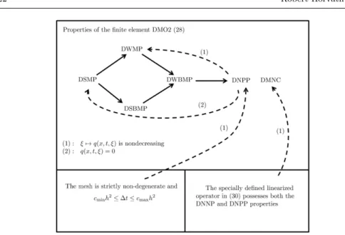
Theorem 10 If the function ξ 7→ q(x, t, ξ) is nondecreasing, then the DNPP (or DNNP) property implies the discrete weak maximum principles DWMP and DWBMP (or discrete weak minimum principles DWmP and DWBmP, respectively) for the DMO2 (24).

Proof In order to apply Theorem 6, we need to show that the condition (W) is satisfied. Consider an arbitrary vector w1 ∈ R^N¯ and a positive constant a. Applying Lemma 1 (i)–(iii), using the nonnegativity of the basis functions and that the functionξ7→q(x, t, ξ) is nondecreasing, we have

S₁^(w1−ae)(w1−ae) =S₁^(w1)w1, S₂^(w1−ae)(w1−ae)≤S₂^(w1)w1,

henceS^(w1−ae)(w1−ae)≤S^(w1)w1.In order to show property (W), let us fix the arbitrary vectors w1 andw2 and the nonnegative numbers a≥b≥0. Using also the properties i) and iii)-iv) in Lemma 1 the required estimation can be carried out as follows:

J(w1−ae, w2−be) =X₁^(w1−ae)(w1−ae)−X₂^(w2−be)(w2−be)

=

_M˜ +θP S^(w1−ae)

(w1−ae)−

_M˜ ₋(1−θ)P S^(w2−be)

(w2−be)

≤_M˜(w1−ae) +θP S^(w1)w1−_M˜(w2−be) + (1−θ)P S^(w2)w2

=X₁^(w1)w1−X₂^(w2)w2−_M˜(a−b)e= X₁^(w1)w1−X₂^(w2)w2−a−b

∆t P M e

=X₁^(w1)w1−X₂^(w2)w2−a−b

∆t e0= J(w1, w2)−a−b

∆t e0,

where we used the equalityP M e=e0.

Theorem 11 Ifq(x, t, ξ)≡0, then the DNPP (or DNNP) property implies the discrete strong maximum principles DMP and DBMP (or discrete strong minimum principles DmP and WBmP, respectively) for the DMO2 (24).

Proof Now we need to show the condition (S). This goes in the same way as the proof Theorem 10 such that the inequalities therein are replaced by equalities.

Remark 5 Note that the conditions of the previous two theorems are the same as those used to guarantee the same implications in the continuous case (see Figure 1).

That is, there is no additional condition in the finite element case.

Corollary 1 In the caseq(x, t, ξ) = 0, if the DMO2 (24)possesses the DNPP property then it fulfills all the discrete maximum principles as well, and if the DMO2 (24) possesses the DNNP property then it fulfills all the minimum principles as well.

4.3 Implication of discrete maximum norm contractivity

Now we give conditions for the relation involving the DMNC property. This relies on a proper linearization of the nonlinear matrix function S^(.) between given ¯z and ˜z, defined as follows:

S^(¯z,˜z)

ij:=

Z

Ω

A˜(x, t,∇z¯_h,∇˜z_h)∇φj· ∇φidx+ Z

Ω

˜

r(x, t,¯z_h,z˜_h)φjφidx.

(25) Theorem 12 Let us suppose that

(I) the functionξ7→q(x, t, ξ)is nondecreasing, and

(L) for any two fixed discrete mesh functionsw¯andw, the mesh operators defined˜ as

(Lw,_¯w˜[v])ⁿ= ( ˜M+θP S^{( ¯wn,w˜n)})vⁿ−( ˜M−(1−θ)P S^{( ¯wn−1,w˜n−1)})vⁿ⁻¹ (26) (n= 1, . . . , n_T), where S^(.,.) stands for the linearized matrix function defined above, possess both the DNNP and DNPP properties.

Then the DMO2 (23)possesses the DMNC property.

Proof We have to show that under the assumptions of the theorem the assumptions (W=) and (L) in Theorem 9 are satisfied. Condition (W=) can be shown in a similar way as condition (W) in Theorem 10, using the fact thata=b.

It is left to show that the condition (L) of this theorem implies the condition (L) in Theorem 9. Thus we have to show the equalityLw,¯w˜[ ¯w−w˜] =D[ ¯w]−D[ ˜w], whereD is the DMO2 defined in (24). In view of equalities (10) and (12), for any two vectors ¯z,z˜∈R^N¯ we have

S^(¯z,˜z)(¯z−˜z)

i=

N¯

X

j=1

S^(¯z,z˜)

ij(¯z_j−z˜_j)

= Z

Ω

A˜(x, t,∇z¯_h,∇˜z_h) (∇z¯_h− ∇˜z_h)· ∇φ_idx+ Z

Ω

˜

r(x, t,z¯_h,˜z_h) (¯z_h−˜z_h)φ_idx

= Z

Ω

(K(x, t,∇z¯_h)−K(x, t,∇z˜_h))· ∇φidx+ Z

Ω

(q(x, t,z¯_h)−q(x, t,˜z_h))φ_idx

= Z

Ω

(A(x, t,∇¯zh)∇¯zh−A(x, t,∇˜zh)∇˜zh)· ∇φidx +

Z

Ω

(r(x, t,z¯_h) ¯z_h−r(x, t,˜z_h) ˜z_h)φidx=

S^(¯z)z¯−S^(˜z)˜z

i.

Thus we obtain that (L_w,¯w˜[ ¯w−w˜])ⁿ

=

M˜ +θP S^{( ¯wn,w˜n)}

( ¯wⁿ−w˜ⁿ)−

M˜ −(1−θ)P S^{( ¯wn−1,w˜n−1)} w¯ⁿ⁻¹−w˜ⁿ⁻¹

= ˜M( ¯wⁿ−w˜ⁿ) +θP

S^{( ¯wn)}w¯ⁿ−S^{( ˜wn)}w˜ⁿ

− M˜

¯

wⁿ⁻¹−w˜ⁿ⁻¹

−(1−θ)P

S^{( ¯wn−1)}w¯ⁿ⁻¹−S^{( ˜wn−1)}w˜ⁿ⁻¹

=

M˜ +θP S^{( ¯wn)}

¯ wⁿ−

M˜ −(1−θ)P S^{( ¯wn−1)}

¯ wⁿ⁻¹

−

M˜ +θP S^{( ˜wn)}

˜ wⁿ−

M˜ −(1−θ)P S^{( ˜wn−1)}

˜ wⁿ⁻¹

= (D[ ¯w]−D[ ˜w])ⁿ (n= 1, . . . , n_T), which completes the proof.

4.4 Ensuring the DNNP–DNPP properties

In the above we have seen that under certain conditions the DNNP or DNPP implies the other studied properties for the DMO2 (24). Now we give conditions to ensure that DNNP and DNPP hold themselves. Altogether, in this way we can also ensure the validity of all the qualitative properties for the finite element mesh operator.

4.4.1 The general case

Definition 3 A finite element meshT_h is called strictly non-degenerate with re- spect to the basis functionsφ1, . . . , φN¯ and the coefficient functionsKandqof the operator (1) (or shortly strictly non-degenerate), if the following condition holds.

For anyi= 1, . . . , N,j= 1, . . . ,_N¯ andi6=j, whenever the basis functionsφ_i and φj have overlapping support, we have

S⁽_ij^z)= Z

Ω

(A(x, t,∇zh)∇φj· ∇φi+r(x, t, z_h)φ_jφ_i) dx <0 (27) for all vectorsz∈R^N¯, whereAandrare the functions defined in (11) and (13) with the coefficient functionsKandq, respectively, and where we denotezh=

N¯

P

k=1

zkφk.

Remark 6 When K(x, t,∇u) = ∇u andq = 0 then for piecewise linear elements on triangular meshes the strict non-degenerateness means the well-known acute angle condition: all angles of the triangles in the triangulation must be less then π/2. For bilinear elements on rectangular mesh the property means the strict non- narrowness of the rectangles. Such geometric conditions can be used to ensure (27) in the general case as well, as will be illustrated by Theorem 14 below.

Now we are ready to give sufficient conditions for the DNNP and DNPP prop- erties of the DMO2 (24).