Evolving Computationally Eﬃcient Hashing for Similarity Search

(1)

Similarity Search

David Iclanzan¹, Sándor Miklós Szilágyi², and László Szilágyi^1,3

1 Faculty of Technical and Human Sciences, Sapientia University, Tˆargu Mure¸s, Romania

2 Department of Informatics, Petru Maior University, Tˆargu Mure¸s, Romania

3 John von Neumann Faculty of Informatics, ´Obuda University, Budapest, Hungary david.iclanzan@gmail.com

Abstract. Finding nearest neighbors in high-dimensional spaces is a very expensive task. Locality-sensitive hashing is a general dimension reduction technique that maps similar elements closely in the hash space, streamlining near neighbor lookup.

In this paper we propose a variable genome length biased random key genetic algorithm whose encoding facilitates the exploration of locality- sensitive hash functions that only use sparsely applied addition operations instead of the usual costly dense multiplications.

Experimental results show that the proposed method obtains highly efficient functions with a much higher mean average precision than standard methods using random projections, while also being much faster to compute.

Keywords: Locality-sensitive hashing·Optimal design·Genetic algorithms·Variable length representation

1 Introduction

The objective of nearest neighbor search or similarity search is to find the item that is closest to what has been queried, from a search (reference) database.

Closeness or proximity is evaluated by some distance measure and the item found is called nearest neighbor. If the reference database is very large or the distance computation between the query and database item is costly, finding the exact nearest neighbor is often not feasible computationally. This has fuelled great research efforts towards an alternative approach, the approximate nearest neighbor search, which proves to be not only more efficient, but also sufficient for many practical problems.

Hashing is a popular, widely-studied solution for approximate nearest neighbor search [11], locality sensitive hashing [3] [8] and learning to hash are the two main classes of hashing algorithms. Locality sensitive hashing (LSH) is data- independent. It has been adopted in many applications, e.g., fast object detection [6], image matching [4]. Learning to hash is a data-dependent hashing approach.

It learns hash functions for specific types of data or datasets, providing a short

(2)

encoding of the original data with the property that the nearest neighbor search result in the hash coding space are also close to the query in the original space [10].

In a recent work [5] the authors showed that a computationally efficient hashing method based on sparse random binary projections has strong distance preserving properties. While the sparse tags can be computed efficiently, their big size prevents a fast nearest neighbor search in the hash space.

In this paper we develop hash function instances based on similarly efficient sparse binary projections. However, instead of a long sparse binary tags the method returns short tags that contain a combination of indices. For nearest neighbor search in the hash space the Jaccard distance is used. Instead of relying on random projections we propose a method for learning the best performing projections using a new random key Genetic Algorithm (GA) that can handle variable length genomes. The new method is used to efficiently explore the sparse binary projection hash functions space, searching for solutions that are both short, therefore very efficient to compute, and also provide high precision for nearest neighbor search.

2 Overview

2.1 Nearest Neighbor Search and Hashing

Nearest neighbor search (NNS) is the optimization problem of locating in a particular space the point that is closest to a query point. To measure closeness or proximity, most commonly a dissimilarity function is used which maps the less similar pair of points to larger values.

The term “locality-sensitive hashing” (LSH) originates from 1998, denoting a “randomized hashing framework for efficient approximate nearest neighbor (ANN) search in high dimensional space. It is based on the definition of LSH family H, a family of hash functions mapping similar input items to the same hash code with higher probability than dissimilar items”[11]. Multiple commu- nities from science and industry alike have been studying LSH, with focus on different aspects and goals.

The theoretical computer science community developed different LSH fami- lies for various distances, sign-random-projection (or sim-hash) for angle-based distance [3], min-hash for Jaccard coefficient [2] explored the theoretical bound- ary of the LSH framework and improved the search scheme.

Learning to hash approaches revolve around the following concepts: the hash function, the similarity in the coding space, the similarity measure in the input space, the loss function for the optimization objective, and the optimization technique. Linear projection, kernels, spherical function, (deep) neural networks, non-parametric functions etc. can all be used as hash functions.

In this paper for the hash function we use sparse binary projections, the similarity measure in the input space is the Euclidean distance while the one in the coding space is the Jaccard distance. The optimisation technique used is an extension of BRKGA, for which we provide an overview in the following.

(3)

2.2 Random Key Genetic Algorithms

A class of random key genetic algorithms (RKGA) was first introduced by Bean [1] for solving combinatorial optimization problems. In a RKGA, chromosomes are encoded as strings, vectors, of random real numbers in the interval [0,1].

Chromosomes, on the other hand, represent solutions to the combinatorial optimization problem for which an objective value or fitness can be computed.

The translation from chromosomes to solutions and fitness is done by a problem dependent, deterministic algorithm called decoder.

The initial population is created randomly by generatingpvectors, wherep is the population size. Each gene of each individual is independently, randomly sampled from the uniform distribution over [0,1]. In the next step the fitness of each individual is computed (by the decoder) and the population is divided into two groups: a smaller group of p_e elite individuals (those with the best fitness values), and the rest,p−penon-elite individuals).

The population evolves into new generations based on a number of princi- ples. First, all the elite individuals are copied unchanged from generation t to generationt+ 1, resulting in a monotonically improving heuristic.

Mutation in Evolutionary Algorithms is usually used for exploration, enabling the method to escape from entrapment in local minima. In RKGA alleles are not mutated, however, at each generation a numberpmof mutants are introduced into the population the same way that an element of the initial population are generated (i.e. randomly from the uniform distribution). Havingp_eelite individuals andp_mmutants in populationt+ 1,p−p_e−p_madditional individuals need to be produced to maintain the same population sizepin generationt+ 1.

This is done by the process of mating, where two parents are selected from the entire population and a new offspring is created by crossover. The crossover is repeatedly applied until the size of population reachesp.

A biased random key genetic algorithm, or BRKGA [7], differs from a RKGA in the way parents are selected for crossover. Each offspring is generated by mating an elite individual with a non-elite one, both taken at random. The bias can be further reinforced by the parametrized uniform crossover [9] and the fact that one parentis always selected from the elite group.

BRKGA searches the continuous n-dimensional unit hypercube (representing the populations), using the decoder to translate search results in the hypercube to solutions in the solution space of the combinatorial optimization problem.

The method and the unbiased variant differ in how they select parents for mating and how crossover favours elite individuals. Offsprings produced by the BRKGA have a higher chance inheriting traits of elite solutions. This seemingly small difference most of the times has a large impact on the performance of these variants. BRKGAs have a stronger exploitation power and tend to find better solutions faster than RKGAs.

(4)

3 Material and Methods

3.1 Distance Preserving Sparse Projections

In [5] it is shown that uniformly distributed, random sparse binary projections preserve neighborhood structure if the number of projections m is sufficiently large.

For the data-dependent hashing, we wish to learn the minimal number of projectionsmneeded and the most discriminatory sparse projections.

Letx∈R^d denote an input that needs to be hashed.y= (y₁, . . . , y_m)∈R^m projections are computed as

y_i= X

j∈Pi

x_j (1)

where Pi is a projection vector defining which components from xare summed for thei-th projection.

The hash is formed by retaining the indexes of thekhighest scoring projections:Z = (z1, . . . , zk)∈Z^kwhere for allzi it holds thatyz_i is one of the largest entries iny.

We use the Jaccard distance to measure how close two hashesZ1andZ2are to each-other:

d_J(Z₁, Z₂) = 1−J(Z₁, Z₂) =|Z₁∪Z₂| − |Z₁∩Z₂|

|Z1∪Z2| (2) For computing a discrete bin index, where one can store similar items for fast reference, we can exploit the fact the computed tags represent a combination of k elements taken from {1, . . . , d}. The combinatorial number system of degree k defines a correspondence between natural numbers and k-combinations. The number N corresponding to a combinationZ= (z_k, . . . , z₂, z₁) is:

N = zk

k

+· · ·+ z2

2

+ z1

1

(3)

3.2 Biased Variable Length Random Key Genetic Algorithm

BRKGA is restricted to searching a continuous n-dimensional unit hypercube, therefore it is not suitable for exploring open-ended design spaces.

For our problem, the optimal number of projections m and the size of the projection vectorsP_imust be determined by the learning algorithm. The method has to explore solutions of various complexities, that cannot be efficiently encoded in a unit hypercube of fixed size.

To enable an efficient exploration of different solution complexities, we extend the BRKGA framework with the following modifications:

– Each chromosome begins with a fixed number of so called interpreter or signalling alleles that can carry information on the complexity of the encoded solution, enabling the decoder to interpret the random keys differently for separate solution classes.

(5)

– Genomes can have various lengths, and they can be as long or as short as needed, to encode highly complex solutions or contrary, simple ones, like the empty set.

– A new 2-parents 2-offsprings crossover operator that can change genome lengths.

– A re-encode operator that can “translate” alleles between different genomes by analysing their interpreter alleles.

The new method, the Biased Variable Length Random Key Genetic Algo- rithm (BVLRKGA), is detailed in the following subsections.

3.3 Interpreter Alleles and Encoding

A solution for the proposed hash model must encode the number of projections mand the projection vectorsPi. Assuming an upper boundθfor the number of projections, and knowing that the elements of the projection vectors are integer numbers between 1 anddthe following encoded can be used.

The first allele on each chromosome is reserved for encoding m. The unit interval is partitioned in θ subintervals of size 1/θ, the upper bound of each subinterval being bi = i/θ, i∈ {1, . . . , θ}. For r ∈[0,1] the first bi ≥r defines the number of projections:m(r) =dr×θe.

The rest of the genes encode elements of the projection vectors. By dividing each subinterval [b_i−1, b_i) assigned to a projection ind subintervals, we reserve a smaller subinterval for each index from {1, . . . , d}. To decode a random key r∈[0,1] first we compute in which projection it encodes an index:

i(r) = 1 +bm(r)×rc (4)

then we compute the index itself:

j(r) = 1 +b(r−(i(r)−1)×m(r))×m(r)×dc (5) For this problem, the order of the genomes is irrelevant, each random key is decoded the same way, independently of its position.

There is no upper bound on the genome length as each index in each projection vector can appear any number of times. In such cases those x_j(r) elements are summed multiple times, hence the number of times they appear in a solution can be regarded as the weight assigned to that dimension.

This encoding can also represent the empty solution when there are no genes besides the interpreter ones. The decoder must take this into account and assign a proper fitness value for empty solutions (usually−inf, 0 or + inf).

3.4 Biased Variable Length Crossover

BRKGA uses a parametrised uniform crossover [9] where alleles from an elite parent are inherited with a higher probability. This operator produces a fixed length offspring, therefore is not suited for variable length encodings.

(6)

We propose a new biased crossover operator where 2 offsprings of potentially various lengths are produced. Each allele from each parent can be inherited by both offsprings with different probabilities. The key is in setting up the probabilities in such a way that i) offsprings are more likely to inherit alleles from the elite parent; ii) the sum of offsprings genome lengths is a random variable whose expected value equals the sum of parents genome lengths. By ii) the crossover is not inherently biased toward in producing shorter or longer offsprings, it produces both with certain variance. The mean average length of offsprings and parents is the same after crossover. It is the role of the selection operator to favour shorter or longer solutions on average.

The crossover operation’s steps are detailed in Alg. 1.

Algorithm 1: Biased variable length crossover Data:elite and other parents:elite,indiv Result:two offsprings:o1,o2

1 eliteBias = 0.2 ; // set up the bias that favours the inheritance of genomes from the elite parent

/* compute probabilities of inheritance */

2 eliteP1 = eliteBias + rand*(1-eliteBias); eliteP2 = (1-eliteBias) -eliteP1;

3 indivP1 = rand*(1-eliteBias); indivP2 = (1-eliteBias) -indivP1;

/* inherit the interpreter alleles from one of the parents */

4 o1 ←elite.interpreterAlleles();o2 ←indiv.interpreterAlleles();

/* inherit the genes according to the 4 probabilities */

5 foreachallele∈elite.randomKeyAlleles()do

6 if rand<eliteP1 then

7 o1.addAllele(allele);

8 if rand<eliteP2 then

9 o2.addAllele(reenc(allele,indiv.interpreterAlleles());

10 foreachallele∈indiv.randomKeyAlleles()do

11 if rand<indivP1 then

12 o1.addAllele(reenc(allele,elite.interpreterAlleles());

13 if rand<indivP2 then

14 o2.addAllele(allele);

The elite bias variable is an element of [0,1] and controls how much the genes of the elite parents are favoured. A value of 0 means that there is no bias while a value of 1 restricts the inheritance only to the genes of the elite individual. The value 0.2 from the listing will result in the offsprings inheriting on average 60%

of their alleles from the elite parent.

The first offspring inherits the interpreter genes on the elite parent while the second inherits from the other individual. As they use different interpretations of random keys, we must make sure then when a allele is inherited from a parent that uses a different solution design, the meaning is preserved. Therefore, a re-

(7)

encoding happens, where the allele is decoded and if possible remapped in the solution space of the offspring. In cases when this is not possible, for example the to be inherited allele encodes an index in the 1000-th projection, while the offspring works with less than 1000 projections, the allele is discarded.

3.5 BVLRKGA

The proposed method uses an elitist approach but there are some notable differ- ences compared to other random key GA. As discussed in the previous section, crossover produce two offsprings of varying lengths. Also, in BVLRKGA we don’t restrict crossover to be between elite and non-elite individuals. While the first parent is always an elite the second one is randomly chosen. This allows mating between elite individuals, that enables the rapid adaptation of ideal genome length in the elite subpopulation. If selection favours short genomes, mating two elite short genomes will produce even shorter solutions with higher probability than mating a short and a long genome. The converse is also true, if long genomes perform better.

In this work, for the hash learning task, random solutions are built by first randomly choosing a projection number m between the hash length k and an upper boundθ=2000. In a second step a spareness factorγ∈[³_d,_d⁹] is randomly chosen, then we decide for each projection if each input dimension index is included in the vector, by flipping aγ-loaded coin. After encoding,mis implicitly encoded in the interpretation allele, while the sparseness is indirectly reflected in the genome length.

4 Experiments

For the experiments, we used a population size of 100 individuals and the evolution was performed over 100 generations. The proportion of elite individuals in the next population was set to p_e = 0.2. The fraction of the population to replaced by mutants was set top_m= 0.4. Therefore, the fraction of the new population obtained by crossover is 1−p_e−p_m= 0.4. For crossover the parameter eliteBias= 0.2. Each experiment was run 10 times.

4.1 Genome Length Adaptation

In a first experiment we checked how fast BVLRKGA can grow or shrink genomes to converge to an optimal target length under ideal selection pressure. The abso- lute difference between genome length and target length was used as fitness, in a minimisation problem context. While most real-world problems will not have a noise free, unimodal feedback regarding the lengths of the solutions, these experiments are very useful in helping assess the effectiveness of the proposed operators in providing solutions of various lengths.

In a first test we set the random individual seeder to build solutions of length 1000, while the best solution is the empty one. Therefore by exploiting the

(8)

0 5 10 15 20 25 30 35 Generations

0 100 200 300 400 500 600 700 800 900 1000

Fitness = abs(1000 - genome length)

Genome length increase under selection pressure

Avg. length of e.i. (10 run avg.) Best individual - run #1 Best individual - run #2 Best individual - run #3 Best individual - run #4 Best individual - run #5 Best individual - run #6 Best individual - run #7 Best individual - run #8 Best individual - run #9 Best individual - run #10

0 5 10 15 20 25

Generations 0

100 200 300 400 500 600 700 800

Fitness = genome length

Genome length reduction under selection pressure Avg. length of e.i. (10 run avg.) Best individual - run #1 Best individual - run #2 Best individual - run #3 Best individual - run #4 Best individual - run #5 Best individual - run #6 Best individual - run #7 Best individual - run #8 Best individual - run #9 Best individual - run #10

a) b)

Fig. 1.Under selection pressure BVLRKGA is able to quickly reduce (a) and increase (b) the genome length of the best solutions.

crossover and selection the method will eliminate alleles gradually. Fig. 1a) de- picts the results of the 10 runs. We can see that the average chromosome length of the elite individuals quickly drops in only 15 generations. Every run reached the empty solution in 24.7 generations on average, while the longest run required 32 generations.

In a second setup we experimented with the converse problem, increasing the genome length beyond what the random individual seeder provides. Here the seeder returned solutions of length 50, while the target solution length was set to 1000. A twentyfold increase in genome length in needed to reach the ideal solution length. The results of 10 runs are shown in Fig. 1b). Again, every run found a best solution, on average in 40.2 generations, the longest run requiring 75 generations to find a solution with a length of exactly 1000. This problem was harder for the BVLRKGA because the optimisation could overshoot, generating solutions with a length beyond 1000, while in the first setup undershooting was not possible.

4.2 Learning to Hash

For testing the BVLRKGA ability to learn hash function we used the MNIST⁴ dataset that contains handwritten digits encoded as 28×28 pixel images (d= 28×28 = 784). We followed the same procedure from [5], using from the dataset a subset of 10.000 vectors, that we pre-processed to have zero mean.

During 4 experiments we evolved models that produced hash tags of lengths k∈ {4,8,16,32}.

For a candidate hash model we first calculated the average precisions (AP:

average precision at different recall levels) by predicting the nearest 200 vectors for a set of query vectors. During the optimisation, this was done by randomly choosing 200 query vectors from the 10.000, each time an evaluation was needed.

4 http://yann.lecun.com/exdb/mnist/

(9)

Averaging over the 200 AP values gives the mean average precision (MAP) of the hash model.

For computing the fitness of a candidate hash model we also took into account the length of the genome:

f itness(c) =M AP(c) +min(0,1000×M AP(c)−bt_k

length(t) ) (6)

The reasoning behind the fitness function is that once a solution reaches a certain precision, compactness (implicitly low computational cost) of the model is rewarded. The bonus thresholds btk ={0.1,0.2,0.3,0.45} were set high enough to reward compactness, shorter solutions once the MAP of the solution is higher as the one of dense projection based LSH functions.

0.1 0.11 0.12 0.13 0.14 0.15 0.16 0.17

MAP 0

100 200 300 400 500 600 700

Genome length

MAP vs genome length - hash length 4 Best individual - run #1

Best individual - run #2 Best individual - run #3 Best individual - run #4 Best individual - run #5 Best individual - run #6 Best individual - run #7 Best individual - run #8 Best individual - run #9 Best individual - run #10

0.21 0.22 0.23 0.24 0.25 0.26 0.27 0.28

MAP 0

500 1000 1500 2000 2500 3000

Genome length

0.28 0.3 0.32 0.34 0.36 0.38 0.4

MAP 0

100 200 300 400 500 600

Genome length

0.46 0.47 0.48 0.49 0.5 0.51 0.52

MAP 0

1000 2000 3000 4000 5000 6000

Genome length

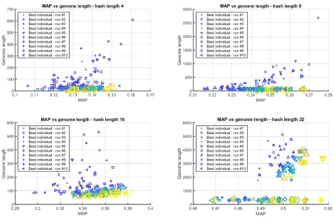
Fig. 2.Development of the two optimisation criteria, MAP and solution length.

The evolution over 100 generations of the best individual is depicted in Fig.

2 for each hash lengthkand each of the 10 runs. The size and color intensity of the markers are proportional to the generation numbers. Small and dark markers correspond to early generations, while individuals depicted from later generations are displayed with a linearly increasing marker size and lighter colors. The scatter plots depict the two relevant metrics in the computation of the fitness, MAP and genome lengths. For hash lengths k ∈ {4,8,16} we can observe the same trend: in early generations the genome lengths are large but with time both the compactness and precision is improved. The genome length is drastically reduced, the biggest markers corresponding to the last generations from each run are very close tox-axis.

(10)

Fork = 32 we can observe two clusters for the final generation markers.In some runs the method is not able to reduce the length of the best solution while also keeping the precision high. These final solutions have genome lengths around 3000. In other runs BVLRKGA is able to find very compact hashes, encoded in genomes with lengths between 200-300, while also keeping MAP above 0.5.

Because all final solution are well above the bonus thresholdb32 = 0.45 we suspect that in some runs the genome lengths are not reduced because the bonus reward is to small and does not compensate the drop in MAP for a shorter solution. This can be mitigated by emphasising, rewarding more the compact solutions.

0 20 40 60 80 100

Generations 0

0.5 1 1.5 2 2.5 3

Fitness / MAP

Mean fitness and MAP values - hash length 4 STD fitness

Mean fitness STD MAP Mean MAP

0 20 40 60 80 100

Generations 0.2

0.4 0.6 0.8 1 1.2 1.4 1.6

Fitness / MAP

0 20 40 60 80 100

Generations 0

0.5 1 1.5 2 2.5

Fitness / MAP

0 20 40 60 80 100

Generations 0.45

0.5 0.55 0.6 0.65 0.7 0.75

Fitness / MAP

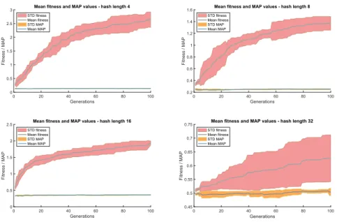
Fig. 3.Fitness development.

Fig. 3 presents the average fitness and MAP values of the best individuals, over the 100 generations. The fitness increases with a much bigger slope than the MAP curve, meaning that the fitness improvements mostly came from the BVLRKGA discovering shorter solutions that do not compromise precision. For k = 32 we can again observe that the standard deviation of the fitness is very large. This comes from the fact that for some runs the fitness curve stayed very close of the MAP, as the genome lengths were high, the compactness bonus was small. In other runs by finding short high-quality solutions, the fitness curve was much higher than the MAP curve.

The details of the best solution found fork= 32 is shown in Fig. 4. As during optimisation the MAP is computed for 200 random queries, we recomputed the

(11)

MAP: 0.5244, length: 222, m: 199, density: 0.0014

5 10 15 20 25

Fig. 4.The pixel locations used by the best model obtained fork= 32.

MAP by querying and averaging al 10.000 images. The solution has a M AP of 0.5244, it uses 222 out thed= 768 input pixels to computem= 199 projections.

The pixels that are part of projection sets with the same size were depicted with the same color in the figure. There is one projection set containing 5 pixel indices (brightest pixels in the figure) and two sets of size 4. Only 31 projection set sizes have more than 1 element. It is interesting to note that the projection sets are mutually exclusive, there is no pixel input that is used in more than one projection.

In order to check if the high MAP value is a results of this very sparse model, with short projections or the location of the inputs discovered by the BVLRKGA has also a big influence, we performed the following experiment: 10.000 random models were generated, using the same parameters,m= 199 projections and a density of 0.001423 to obtain on average 222 indices. The average MAP values of these models was 0.4481 and none of them reached a MAP value of 0.5. The experiments show that even if the model parameters are fixed it is very hard to replicate the performance of the proposed method with random sampling.

Therefore, we conclude that BVLRKGA not only explores the model design space efficiently, obtaining very compact solutions, but it also combines mean- ingfully solutions to reach models with high MAP.

5 Conclusions

We proposed a method for obtaining computationally efficient locality sensitive hash functions based on sparse binary projections. The tags are not binary, instead they encode a short combination of indices. For these tags, nearest neighbor search in the hash space can is performed by using the Jaccard distance.

The paper introduces the Biased Variable Length Random Key Genetic Al- gorithm (BVLRKGA) that is able to explore a solution design space in order to find the appropriate solution complexity that provide both high precision and good computational efficiency - short solutions. By using a crossover operator that can produce offsprings of different lengths and enabling mating between

(12)

elite individuals, under the appropriate fitness pressure the method can quickly converge to an ideal genome length.

The method was used to find computationally very efficient locality-sensitive hash functions for the MNIST dataset. Hashing with the evolved solutions is order of magnitudes faster than standard LSH functions that use many multiplications. The evolved functions only require a few addition operations to compute.

Acknowledgments

This paper was partially supported by the Sapientia Institute for Research Pro- grams (KPI). The work of Sándor Miklós Szilágyi and László Szilágyi was ad- ditionally supported by the Hungarian Academy of Sciences through the János Bolyai Fellowship program.

References

1. Bean, J.C.: Genetic algorithms and random keys for sequencing and optimization.

ORSA J. Comput.6(2), 154–160 (1994)

2. Broder, A.Z.: On the resemblance and containment of documents. In: Proceedings of Compression and Complexity of Sequences. pp. 21–29. IEEE Computer Society (1997)

3. Charikar, M.S.: Similarity estimation techniques from rounding algorithms. In:

Proceedings of the 34th Annual ACM Symposium on Theory of Computing. pp.

380–388. ACM, New York, NY, USA (2002)

4. Chum, O., Matas, J.: Large-scale discovery of spatially related images. IEEE Trans.

Pattern Anal. Mach. Intell.32(2), 371–377 (2010)

5. Dasgupta, S., Stevens, C.F., Navlakha, S.: A neural algorithm for a fundamental computing problem. Science358(6364), 793–796 (2017)

6. Dean, T., Ruzon, M.A., Segal, M., Shlens, J., Vijayanarasimhan, S., Yagnik, J.:

Fast, accurate detection of 100,000 object classes on a single machine. In: IEEE Conference on Computer Vision and Pattern Recognition (CVPR). pp. 1814–1821.

IEEE (2013)

7. Gon¸calves, J.F., Resende, M.G.C.: Biased random-key genetic algorithms for combinatorial optimization. J. Heuristics17(5), 487–525 (2011)

8. Indyk, P., Motwani, R.: Approximate nearest neighbors: towards removing the curse of dimensionality. In: Proceedings of the 30th Annual ACM Symposium on Theory of Computing. pp. 604–613. ACM (1998)

9. Spears, W., DeJong, K.: On the virtues of parameterized uniform crossover. In:

Proceedings of the Fourth International Conference on Genetic Algorithms. pp.

230–236 (1991)

10. Wang, J., Zhang, T., Song, J., Sebe, N., Shen, H.T.: A survey on learning to hash.

IEEE Trans. Pattern Anal. Mach. Intell.40(4), 769–790 (2018)

11. Wang, J., Shen, H.T., Song, J., Ji, J.: Hashing for similarity search: A survey.

CoRRabs/1408.2927(2014)