Efficiently parallelised algorithm
to find isoptic surface of polyhedral meshes
Ferenc Nagy
Faculty of Informatics, University of Debrecen, Hungary Doctoral School of Informatics, University of Debrecen, Hungary
nagy.ferenc@inf.unideb.hu Submitted: February 8, 2020
Accepted: May 1, 2020 Published online: May 14, 2019
Abstract
The isoptic surface of a three-dimensional shape is defined in [1] as the generalization of isoptics of curves. The authors of the paper also presented an algorithm to determine isoptic surfaces of convex meshes. In [9] new searching algorithms are provided to find points of the isoptic surface of a triangulated model inE3. The new algorithms work for concave shapes as well.
In this paper, we present a faster, simpler, and efficiently parallelised version of the algorithm of [9] that can be used to search for the points of the isoptic surface of a given closed polyhedral mesh, taking advantage of the computing capabilities of the high-performance graphics cards and using the benefits of nested parallelism. For the simultaneous computations, the NVIDIA’s Compute Unified Device Architecture (CUDA) was used. Our experiments show speedups up to 100 times using the new parallel algorithm.
Keywords:Isoptic surface, CUDA, Parallel algorithm, Nested parallelism MSC:65D17, 68U07
1. Introduction
The isoptic curves in the Euclidean plane E2 have been widely studied since cen- turies. It is defined as the locus of points, from where a given curve can be seen under a predefined angle (of less than 𝜋). There are well-known results of several doi: https://doi.org/10.33039/ami.2020.05.002
url: https://ami.uni-eszterhazy.hu
167
classical curves [13]. However, the exact calculation of the isoptic curve may be a complicated task. For example, using direct computations, it is only possible to obtain it for low degree Bézier curves [6]. In such difficult cases, the points of the isoptic curve are determined by the appropriate tangents of the given curve, which meet at the given angle.
The isoptics in the three-dimensional space, besides the theoretical results, can also be of great interest in certain applications, which are concerned with the quality or quantity of visibility. However, the extension toE3is not straightforward and the calculations are also getting more complicated. In [8] an algorithm was presented to find the isoptic curve of a Bézier surface to be used as a camera path. Despite the specific case, the exact equations seemed too difficult to solve, even for computer algebra systems. Only the numerical methods can determine the isoptic curve.
In [1], the isoptic inE3is defined as a surface by substituting the two-dimensional viewing angle for the appropriate three-dimensional measure of visibility (solid angle). The authors are also provided a formula and algorithm for convex shapes, but it is possible to solve and plot the isoptic surface only using computer algebra systems. Moreover, it takes around 20–40 minutes to display it, even for simple regular polyhedra. In [9], a faster, general algorithm was presented to determine the isoptic surface of a given polyhedral mesh. These results, including the precise definitions, will be briefly summarized in Section 2.
The latter algorithm is able to find and render the isoptic surface in case of concave objects as well independently of computer algebra systems, but for a mesh with a few hundred polygons, the process still takes several minutes. Our aim is to accelerate the algorithm of [9] to find the isoptic surface within a reasonable time, using general-purpose computing on graphics processing units (GPGPU).
In the following sections, we present the simpler and parallel version of the algorithm. The different levels of parallelism will be discussed separately, in Sec- tion 3 and in Section 4. The running times of the new GPU-based methods will be compared with the original version of the algorithm presented in [9] in Section 5.
2. Previous results
In this section, we recall the notion of the isoptic surface, defined in [1] and briefly describe the earlier sequential algorithm, presented in [9] that obtains the isoptic surface of a closed polyhedral mesh.
The 3D generalization of the isoptics is based on the extension of the two- dimensional measure of angles. The angle at vertex𝐴can be measured by the arc length on the unit circle around𝐴. An appropriate substitution of the arc length in the Euclidean space can be the solid angle [2]:
Definition 2.1. The solid angleΩ𝒮(𝑃)subtended by a surface𝒮is defined as the surface area of the projection of𝒮 onto the unit sphere around 𝑃.
Based on this notion the isoptic surface is defined in [1] as follows:
Definition 2.2. The isoptic surface𝒮𝒟𝛼 inE3 of an arbitrary 3-dimensional com- pact domain𝒟 is the locus of points𝑃 where the measure of the projection of 𝒟 onto the unit sphere around𝑃 is equal to a given fixed solid angle value𝛼, where 0<𝛼<2𝜋.
The algorithm, presented in [9] searches for spatial points around the mesh, where the solid angle is equal to a given value 𝛼. The solid angle is calculated at each point 𝑃 as the area of the projection of the given model on the unit sphere, centered at𝑃. The projection of a polyhedral mesh covers a spherical polygon on the unit sphere, the area of which can be calculated by the following formula:
Ω(𝑃) =𝜃−(𝑛−2)𝜋, (2.1)
where𝑛is the number of the containing vertices and 𝜃is the sum of the angles of the spherical polygon.
After calculating the solid angle, the isoptic surface of the model can be deter- mined by finding the appropriate three-dimensional points, where the solid angle is equal to the given value𝛼. The search for these points is done using the following methods, regarding [9]:
1. brute-force: one can scan the space around the model with a given increment and select the appropriate 3-dimensional points, where the solid angle differs from the given𝛼with a suitable small (error) value.
2. flood-fill: in this search, we test the neighboring positions of a previously found isoptic point. The first point can be determined by shooting a ray outwards from the barycenter of the mesh.
3. spherical: it is based on the search of the first point of the flood-fill method, by shooting rays outwards from the barycenter of the mesh into many directions.
The result of the above algorithms is the point cloud of the isoptic surface of the given mesh. The comparison of the search methods is described in [9]. From the found points the isoptic surface can be constructed as a polygon model using mesh reconstruction algorithms (see Figure 1).
The running time of the algorithm highly depends on the speed of obtaining the spherical contour (and calculating the solid angle) and the swiftness of the used searching method. In Section 3, we present an alternative method to accelerate the computation of the solid angle at point𝑃, using the graphical processing unit (GPU). The steps of the algorithm call special functions that run on the GPU.
In CUDA they are called kernels. Each execution launches a specified number of thread blocks (a group of threads) and each thread performs the operation specified by the kernel function.
Besides the procedure that calculates the solid angle, the used search method can also be accelerated by parallel processing. Therefore, the algorithm to find the isoptic surface requires embedded kernel launches. This solution leads us to use multiple levels of parallelism. In CUDA it is called dynamic parallelism [3]. It enables the threads to create and synchronize new nested work. The new parallel versions of the searching methods will be discussed in Section 4.
Figure 1: Isoptic surface of an airplane model, constructed from point cloud (𝛼=𝜋2, model source: www.cadnav.com)
3. Solid angle computation in parallel mode
Let ℳbe a closed polyhedral mesh given in a half-edge data structure, in which each facetℱ is represented by a list of directed edgesℰ. The vertices of the edges belonging to the same facet are required to be in counterclockwise order to calculate the proper solid angle. Beside the endpoints (V_1[3], V_2[3]), to determine faster the visible edges from a point 𝑃 the normal vector (other_normal[3]) of the other facet that also contains the edge is stored as well:
edge = {
V_1[3] : float ;
V_2[3] : float ;
other_normal[3] : float ; }
Listing 1: Edge data structure
To make the computations easier, one can apply a coordinate transformation to place the origin into the center of the unit sphere (i.e. 𝑃). In this case, during the calculation of the solid angle ofℳat a point𝑃 we project the model onto an origin centered unit sphere.
The algorithm of [9] first determines the spherical boundary of the projection and then computes the spherical area of it. The new method focuses on the calcu- lation of the solid angle, rather than obtaining the spherical contour. The compu- tation requires four steps. At first, one needs to project the edges ofℳ onto the unit sphere, then calculate the spherical angles at all the intersections. After, to summarize the appropriate spherical angles, it is required to find a proper starting point. The last step is the traversing of the consecutive (counterclockwise ordered)
edges at their intersections. It is done by selecting always that edge, which inter- sects the given edge closer to its first vertex or which meet at the same position but has a higher spherical angle at the intersection. Finally, the solid angle is obtained using Eq. (2.1).
The following subsections will describe the steps in detail and specify the tech- nique and data structures needed for the parallelisation. The final pseudo-code of the algorithm is shown in Listing 4.
3.1. Projecting edges
To calculate the solid angle on the unit sphere it is necessary to project the edges of the facets visible from 𝑃. To avoid projecting the edges containing the same endpoints with the opposite direction we project the edges which belong to one facet visible from 𝑃 and to another that hidden from 𝑃. The selection of the appropriate edges is done efficiently, using theother_normal[3]data of Listing 1. In this step, we create a new array 𝒮 that consists of the projected edges, which are great arc segments on the origin centered unit sphere. The elements of𝒮 have the following structure:
spherical_edge = {
A[3] : float ;
B[3] : float ;
dist_from_center : float ; intersection_id[max_int] : integer ;
n_int : integer ;
}
Listing 2: Spherical edge data structure
The projected endpoints A[3] and B[3] remain stored as points of E3. The
dist_from_centeris the distance between B[3] and the projection of the barycenter of ℳ. It is required for the subsequent step of the algorithm but the values are computed in this stage. It can be calculated as spherical or Euclidean distance. To avoid using trigonometric functions, the latter is preferred. The rest of Listing 2 will be explained in the further steps of the algorithm.
It is possible to fill𝒮 in parallel since the faces can be processed independently.
However, for the preceding memory allocation, it is necessary to approximate the expected size of 𝒮 (see max_S in Listing 4). For simplicity, one can multiply the number of facets of ℳ by the number of edges of a facet (which is three in case of triangulated meshes) to obtain a limit of𝒮. However, a better approximation is recommended to preserve the memory. The authors of [5] have made a probabilistic analysis of the expected number of the contour edges with respect to a random viewing direction, which can be used to approximate the size of 𝒮. Therefore, the expected number of the contour edges is calculated by the following formula [5]:
∑︁
𝑒∈ℰ
1−2𝜑𝑒, where𝜑𝑒= 1
2𝜋arccos −𝑛⃗𝑓𝑖·𝑛⃗𝑓𝑗
| −𝑛⃗𝑓𝑖||𝑛⃗𝑓𝑗|. (3.1)
The 𝑛⃗𝑓𝑖 and𝑛⃗𝑓𝑗 are the normal vectors of faces𝑓𝑖 and 𝑓𝑗 ∈ ℱ and the𝜑𝑒 is the probability that the facets incident to𝑒∈ ℰ are both front or both back facets.
In addition, the further steps of the algorithm require the exact size𝑛𝒮 of𝒮, therefore it needs to be counted during the filling. It can be is done using atomic increment operation that reads the value at a specified address of the memory, adds a number to it (in this case one), and writes the result back to the same address.
The atomic means that, it is guaranteed to be performed without interference from other threads [11].
3.2. Calculating intersections
In this step one needs to calculate the spherical angles of all the overlapping edge pairs𝑒and𝑓 of𝒮 at the intersections and when they meet at an opposite endpoint (A[3]𝑒 =B[3]𝑓 or B[3]𝑒 =A[3]𝑓). This stage is done in a brute-force manner, in parallel (consider all pairs of spherical segments and test each pair for intersec- tion). The intersection point of two projected edge is computed using the formula described in [9]. However, there are faster line segment intersection algorithms for GPU (such as [12]), considering the nested parallelisation, the much simpler brute-force manner is recommended.
Besides the spherical angles, the algorithm requires other data as well. If there is an intersection between𝑒and𝑓, we set two elements in the intersection arrayℐ, using the following structure:
intersection = { angle : float ; other_edge : integer ; dist_from_A : float ; }
Listing 3: Intersection data structure
One element, which corresponds to edge 𝑒 stores the spherical angle between 𝑒 and 𝑓. To calculate it (up to 2𝜋), the formula presented in [9] was used. The
other_edgeis the index𝑗of edge𝑓 in𝒮. Thedist_from_Ais the distance between the intersection point and the first endpoint (A[3]) of edge𝑒. It can also be calculated as spherical or Euclidean distance. The other element that corresponds to edge 𝑓 stores the 2𝜋 - angle, the index 𝑖 of 𝑒, and the distance between the intersection point and the first endpoint of𝑓.
The above calculations are processed in parallel, using one thread for each 𝑒 and𝑓 pairs. Theℐ is stored in the global memory as a one-dimensional array. The size of it should be the number of the expected size of the projected edges on the square to avoid array access conflicts. The appropriate indices in ℐ of the element 𝑒and 𝑓 is calculated using their indices 𝑖,𝑗 and the size𝑛𝒮. The position of𝑒 is 𝑛𝒮·𝑖+𝑗 and𝑓 is𝑛𝒮 ·𝑗+𝑖.
The element indices ofℐare also needed to be stored locally in the correspond- ing edge structure (see intersection_id[max_int]in Listing 2). Since one spherical
segment can cross multiple others, it also needs to be stored as an array. The size max_intof it should be estimated previously for the memory allocation. In [5], there is a formula also for the expected number of edge intersections. The detailed calculation of the probability that two edges are crossing with respect to a random viewing direction is described in Section 3. of [5]. To obtain max_int, one needs to find that edge pair that has the highest likelihood. In addition, the coincident endpoints of the edges also need to be considered, since they are also stored as intersections. To take it into account, one needs to find that vertex position, where the most facets meet. The number of the incident facets at this vertex should be added twice to consider the intersection at both endpoints of an edge.
The actual number of the intersections, i.e. the sizen_intof the local array (in Listing 2) is counted similarly as in the case of𝒮, using atomic increment operation.
3.3. Finding the first edge
To begin the traversal of 𝒮 one needs to determine a proper starting spherical segment 𝑒 that is a contour edge of 𝒮. It is selected by its first endpoint A[3]𝑒, which should be the farthest away from the projection𝐶 of the barycenter of ℳ. However, it is also necessary that the vertex of the mesh that corresponds toA[3]𝑒
is visible from𝑃 and not covered by any facet ofℳ. It can be seen, if the spherical arc segment𝐶′A[3]⌢ 𝑒, formed by the antipode of𝐶andA[3]𝑒, does not intersect with any edge of𝒮. The above conditions can also be satisfied by the first endpoint of an interior silhouette of𝒮. Therefore, to obtain a contour spherical segment𝑒, one has to select the edge that has the highest spherical angle^𝐶′B[3]𝑒A[3]𝑒.
Inℐ, besides the intersections, the coincident opposite endpoints are also stored.
Therefore, let us find the farthest endpoint B[3]𝑓 from 𝐶, using dist_from_center
of Listing 2. In this way, the starting edge 𝑒 with the highest spherical angle
^𝐶′B[3]𝑒A[3]𝑒 is found faster since 𝒮 is not processed again because the indices of the possible starting edges are obtained using the localintersection_id[max_int]
array of𝑓.
In this step, the visibility test is processed simultaneously. In the iteration of obtaining the farthest endpointB[3]𝑓 from𝐶′ the spherical arc segment𝐶′B[3]⌢ 𝑓 is tested for intersection with the other edges of 𝒮 in parallel.
3.4. Calculating the sum of the spherical angles
The final task is to summarize the appropriate spherical angles by traversing𝒮 and calculate the solid angle using Eq. (2.1). It can only be done by an iterative loop, that begins with the selected starting arc segment.
One has to go along its intersections using the local array intersection_id[
max_int] of Listing 2 and select the subsequent edge by comparing the distances between its intersections and the first endpoint. The distance values are computed in dist_from_A of Listing 3. The following edge is that, which has the closest in- tersection. Its index is stored in other_edge. If a spherical arc segment has more
than one intersection at the same position (in cases when thedist_from_Avalues are equal) the one with the highest spherical angle needs to be considered.
The search of the minimumdist_from_Aof an edge𝑓 does not necessarily start from zero but from a minimum value, based on where the earlier edge𝑒is connected.
In case of an intersection between𝑒and𝑓 two elements are added toℐ. Each stores the distance from the first endpoint and the cross point. Therefore, the minimum value can be obtained by finding the corresponding members in ℐ. If the index of the intersection element of the edge𝑒in ℐ is 𝑖, then the corresponding element index𝑗ofℐ that belongs to the next edge𝑓 is calculated as𝑛𝒮(𝑖mod𝑛𝑒) + (𝑖/𝑛𝒮), where𝑛𝒮 is the size of𝒮.
The iteration ends when the loop reaches again the first edge. During the traversal, the appropriate spherical angles are added directly to𝜃of Eq. (2.1) since the values are already calculated.
Regarding [5], one contour edge has only a few numbers of intersections (n_int), therefore, it is not necessary to sort them since it can be traversed fast enough iteratively. The complete pseudo-code of the solid angle computation is shown in Listing 4.
4. Search for the isoptic points in parallel mode
In the preceding sections, the new parallel method is described to compute the solid angle and decide when the point 𝑃 in E3 is a point of the isoptic surface of ℳ.
Besides the speed, the simplicity of the algorithm is also important, since we intend to calculate it for multiple points at the same time, using the new parallel search methods. In this case, all the computations to obtain the point cloud of the isoptic surface are embedded into one kernel function call, which entirely handled by the graphical processor. The procedures to calculate the solid angle at the specific 3- dimensional points are nested parallel works. The new approach is efficient because the process is not interrupted by memory management operations. All the required space can be allocated and all the required data can be loaded into the memory previously.
To search for the isoptic points in parallel the following modifications need to be performed:
1. brute-force: one has to divide the space around ℳ, where the points are searched into a discrete set of cubes (see marching cubes in [7]) and process the containing points of the cubes at the same time.
2. spherical: in this case, one can do the search in many directions simultane- ously from the barycenter of the vertices ofℳ. Each thread can process one direction.
Unfortunately, the flood-fill search can not be accelerated using the GPU. In the case of the above methods, the parallelisation was feasible and straightforward.
The main difficulty of the flood-fill algorithm, even in the sequential CPU case is
to keep track of the previously visited positions. In the CPU version, to speed up the process a binary search tree can be used. However, there are also algorithms to build search trees parallel on the GPU (e.g. [10]) along with the new solid angle computation the isoptic surface determination is slower than the CPU version algorithm.
The algorithms running on the GPU are producing the same isoptic surfaces as the CPU versions since the base stages of the algorithms are the same (calculating the solid angle and the search for the three-dimensional points).
R r ·
α 2
Figure 2: Radius𝑅 of the isoptic of the circle
In the case of the brute-force method the space around the model which needs to be traversed can be defined using a minimum bounding sphere ofℳ. The isoptic surface of this enclosing sphere is also a sphere. Its radius𝑅is calculated similarly as the radius of the two-dimensional isoptic of the circle (see Figure 2):
𝑅=𝑟/sin𝛼 2,
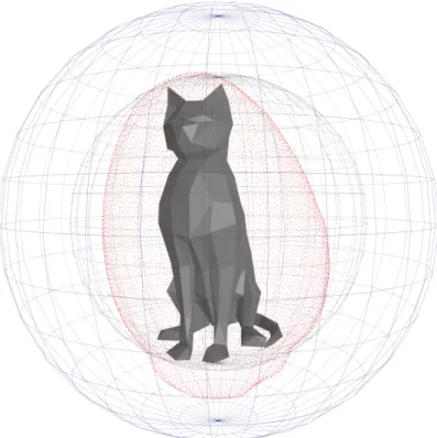
where 𝑟is the radius of the bounding sphere. The radius𝑅 defines the maximum distance from the mesh, where the isoptic points of ℳ are (See Figure 3). This maximum distance can also be used in case of the spherical method to limit the search.
Figure 3: The points (red dots) of the isoptic surface of the cat model are inside the isoptic (blue sphere) of the enclosing sphere
(model source: www.turbosquid.com)
5. Performance analysis
Table 1 shows the execution time of the original CPU-based algorithms of [9] and the new GPU-based methods, using the following parameters: 𝛼= 𝜋2, the size of the traversal step is 0.1, and a point 𝑃 is accepted if the difference between the calculated solid angle at point𝑃 and𝛼is less than2×10−3(error). All the tested models are scaled to have radius𝑟= 5of the bounding sphere, which is calculated as the distance of the farthest vertex from the barycenter of the mesh. Therefore the same radius𝑅= 5/sin(𝜋/4)was used for all the meshes. The experiments were run on an Intel Core i7-7700HQ and Geforce GTX 1050 Ti with CUDA version 10.1. The algorithms were using single-precision arithmetic. The results can be seen in Figure 4. The isoptic surfaces around the tested objects are displayed as wireframe models created from the found point cloud using mesh reconstruction algorithm [4].
The execution times are generally increasing according to the complexity of the
Model Brute-force Spherical Sequential Parallel Sequential Parallel
Stanford Bunny 499.1 10.6 24.2 0.9
F: 128, V: 66
Cat 2279.9 36.5 117.4 2.9
F: 428, V: 216
Moose 4233.7 92.2 228.9 8.8
F: 747, V: 376
Airplane 6449.4 63.8 418.3 5.1
F: 910, V: 529
Elephant 9185.6 163.5 453.5 13.6
F: 1492, V: 779
Table 1: Execution times (in seconds) of the previous sequential and the new GPU-based parallel searching algorithms (𝛼 = 𝜋2, step size = 0.1, solid angle error = 2×10⁻³, F and V are the numbers of the faces and
vertices of the models)
meshes. However, in the case of the airplane model, which consists of more faces than the moose model, the parallel algorithm finds the isoptic surface within a shorter time. The reason behind is the number of the threads running in parallel.
The expected size of𝒮is estimated using Eq. (3.1). This calculation is based on the probability that both facets sharing the same edge are front faces with respect to a random viewing direction. On the wings of the airplane model, there are numerous coincident front facets from many positions, which imply the small number of the expected contour edges. Therefore, more threads can search in parallel because the fewer number of contour edges indicates the larger size of the marching cubes. It causes lower execution times for the airplane model in case of the GPU algorithms.
Figure 4: Isoptic surfaces of the tested models (Stanford Bunny, a moose and an elephant), constructed from point cloud (𝛼=𝜋2, model sources: graphics.stanford.edu/data/3Dscanrep, www.
cadnav.com)
6. Summary
As can be seen from Table 1, the search of the isoptic surface is highly accelerated using the new parallel algorithms. In case of simple meshes, it effects greatly for the whole isoptic surface obtaining process. However, in case of complex meshes, the parallelism of the searching methods is limited, because the solid angle computation consumes more GPU resources (memory space and threads as well). Therefore, fewer points are searched in parallel.
To render the isoptic surface of a highly detailed polyhedral mesh (with thou- sands of facets) using the new GPU algorithms can still be time-consuming. A simple way to increase the speed is to search for the spatial isoptic points after the decimation of the given model, because even significant polygon reduction of the mesh can cause only slight decrease of the area of its projection, which is negligible, regarding the acceptance error between the given𝛼and the computed solid angle.
Acknowledgements. This work was supported by the construction EFOP-3.6.3- VEKOP-16-2017-00002. The project was supported by the European Union, co- financed by the European Social Fund.
References
[1] G. Csima,J. Szirmai:Isoptic surfaces of polyhedra, Computer Aided Geometric Design 47 (2016), pp. 55–60,
doi:https://doi.org/10.1016/j.cagd.2016.03.001.
[2] R. Gardner,K. Verghese:On the solid angle subtended by a circular disc, Nuclear In- struments and Methods 93.1 (1971), pp. 163–167,
doi:https://doi.org/10.1016/0029-554X(71)90155-8.
[3] S. Jones:Introduction to dynamic parallelism, Nvidia GPU Technology Conference (GTC), May 2012.
[4] M. Kazhdan,H. Hoppe:Screened Poisson Surface Reconstruction, ACM Transactions on Graphics (TOG) 32.3 (2013), p. 29,
doi:https://doi.org/10.1145/2487228.2487237.
[5] L. Kettner,E. Welzl:Contour edge analysis for polyhedron projections, in: Geometric Modeling: Theory and Practice, ed. by W. Strasser,R. Klein,R. Rau, Springer, 1997, pp. 379–394,
doi:https://doi.org/10.1007/978-3-642-60607-6_25.
[6] R. Kunkli,I. Papp,M. Hoffmann:Isoptics of Bézier curves, Computer Aided Geometric Design 30.1 (2013), pp. 78–84,
doi:https://doi.org/10.1016/j.cagd.2012.05.002.
[7] W. E. Lorensen,H. E. Cline:Marching cubes: A high resolution 3D surface construction algorithm, ACM SIGGRAPH Computer Graphics 21.4 (1987), pp. 163–169,
doi:https://doi.org/10.1145/37402.37422.
[8] F. Nagy,R. Kunkli:Method for computing angle constrained isoptic curves for surfaces, Annales Mathematicae et Informaticae 42 (2013), pp. 65–70.
[9] F. Nagy,R. Kunkli,M. Hoffmann:New algorithm to find isoptic surfaces of polyhedral meshes, Computer Aided Geometric Design 64 (2018), pp. 90–99,
doi:https://doi.org/10.1016/j.cagd.2018.04.001.
[10] N. Nakasato:Implementation of a parallel tree method on a GPU, Journal of Computa- tional Science 3.3 (2012), pp. 132–141,
doi:https://doi.org/10.1016/j.jocs.2011.01.006.
[11] NVIDIA:NVIDIA CUDA C programming guide, 2019.
[12] C. Rüb:Line-segment intersection reporting in parallel, Algorithmica 8.1-6 (1992), pp. 119–
144,
doi:https://doi.org/10.1007/BF01758839.
[13] R. C. Yates:A Handbook on Curves and their Properties, Ann Arbor, J.W. Edwards, 1947, pp. 138–140.
Appendix
float CALCULATE_SOLID_ANGLE(P[3], faces) spherical_edge S[max_S] // max_S approximated n_S = PROJECT_EDGES(*S, faces)
CALCULATE_INTERSECTIONS(S, n_S) float min = float_max
spherical_edge f, first
foreach spherical_edge e of S do
if (e.dist_from_center < min AND IS_VISIBLE(e)) f = e
min = e.dist_from_center endif
endforeach min = 0
spherical_edge C_fB // from the antipode of C to f.B foreach index i of f.intersection_id do
if ((I[i].dist_from_a=length(f)) AND // it is at f.B (spherical_angle(Cf_B, S[I[i].other_edge])>min)) first = S[I[i].other_edge]
min = spherical_angle(Cf_B, S[I[i].other_edge]) endif
endforeach
spherical_edge current_edge = first integer n = 0 // number of traversed edges float theta, min_dist = 0
repeat
integer int_id
float min_angle = 0, max_dist = 2 // Euclidean distance foreach index i of current_edge.intersection_id do
if (((I[i].dist_from_a > min_dist) OR ((I[i].dist_from_a = min_dist) AND
(I[i].angle > min_angle))) AND (I[i].dist_from_a < max_dist)) int_id = i
max_dist = I[i].dist_from_a min_angle = I[i].angle endif
endforeach
theta = theta + I[i].angle
min_dist = I[n_S * (int_id%n_S) + (int_id/n_S)].dist current_edge = S[I[int_id].other_edge]
n = n + 1
until (current_edge != first) return (theta - ((n - 2) * PI)) end CALCULATE_SOLID_ANGLE
Listing 4: Solid angle computation method