38(2011) pp. 37–44
http://ami.ektf.hu
A convexity test for control point based curves ∗
Imre Juhász
Department of Descriptive Geometry, University of Miskolc, Egyetemváros Miskolc, Hungary
agtji@uni-miskolc.hu
Submitted November 15, 2011 Accepted December 06, 2011
Abstract
We study the convexity of curves defined by the combination of control points and blending functions, that are globally controlled. We provide a method using which the convexity of the curve can be determined by the location of one of its control points.
Keywords: convex curve, convexity test, singularity, inflection point, self- intersection, cusp
MSC:65D17, 68U07
1. Introduction
Convexity of curves is an important concept in Computer Aided Geometric Design.
We adopt the following definition of convex curves (see e.g. [4]).
Definition 1.1. A curve is convex if it is (a part of) the boundary of a convex plane figure.
One can find other approaches, such as
• A (directed) plane curve is convex if it is on the same side of its (directed) tangents (cf. [3]).
∗This research was carried out as a part of the TAMOP-4.2.1.B-10/2/KONV-2010-0001 project with support by the European Union, co-financed by the European Social Fund.
37
• A curve is convex, if it is intersected by any hyperplane in at most two points or it lies completely in the hyperplane. (c.f. [5], [1]) Therefore, convex curves are plane curves (lie in two-dimensional planes). This is a bit more restrictive than Definition 1.1, since excludes curves that contain straight line segments.
In [3] there is a comprehensive study on the convexity of directed parametric curves. According to that treatment the same plane curve can be convex or concave depending on its direction.
Based on the more traditional Definition 1.1 we study the global convexity of control point based curves
g(u) =
n
X
j=0
Fj(u)dj, u∈[a, b], (1.1)
where functions{Fi(u)}ni=0 are assumed to be at least twice continuously differen- tiable.
Applying the moving control point concept, we propose a method that provides both a visual aid for interactive convex curve design and a simple convexity check algorithm for all curves defined by the combination of control points and blending functions. In comparison with the already published results, the proposed method is rather intuitive and easy to implement and use.
2. Singularity
We briefly summarize those results of [2] that we will utilize in the sequel. We let control point di, i ∈ {0,1, . . . , n} vary and fix the rest. Separating the fixed and varying parts of (1.1) we obtain
g(u) =Fi(u)di+ri(u), ri(u) =
n
X
j=0,j6=i
Fj(u)dj. (2.1)
We assume that control point di has influence on the shape of the whole curve, i.e. we suppose that the curve is globally controlled. Consequently, the proposed method is not suitable for spline curves, i.e. for locally controlled curves.
Curve
ci(u) =−˙ri(u)
F˙i(u) (2.2)
is called theith discriminant of curve (1.1).
Conditions for singularity are as follows.
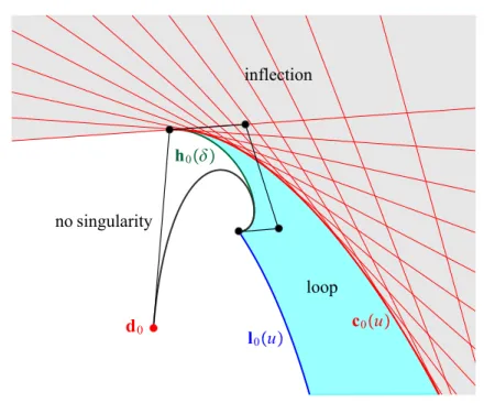
• The locus of control pointdithat results a cusp on the curve (1.1) is theith discriminant (2.2).
• The locus of control pointdi that results a zero curvature point on the curve (1.1) is the region in the plane that is covered by the tangent lines of theith discriminant (2.2).
Figure 1: Singularity regions of a quartic Bézier curve with respect to its control pointd0.
• The locus of control pointdithat results a self-intersection point on the curve (1.1) is the triangular region in the plane bounded by the curves
li(u) =−ri(b)−ri(u)
Fi(b)−Fi(u), u∈[a, b], (2.3) hi(δ) =−ri(a+δ)−ri(a)
Fi(a+δ)−Fi(a), δ∈(0, b−a]
and by theith discriminant (2.2).
These singularities are illustrated in Fig. 1 for a quartic Bézier curve with respect to its control pointd0.
3. Convexity
As is known, if the curve (1.1) shares the variation diminishing property, then any convex control polygon results a convex curve. However, the converse is not true in general.
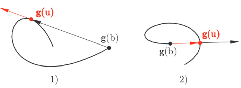
We assume that curve (1.1) has no inflection point, cusp and self-intersection point, i.e. it is free of singularity. Under these circumstances, closed curves (g(a) = g(b)) are convex. In case of open curves, however this is not necessarily true, the two possible types of counterexamples can be seen in Fig. 2.
Figure 2: Singularity free nonconvex open curves.
3.1. Case 1
The left hand side figure of Figure 2 shows that case when a tangent line can be drawn from the endpointg(b)to the curve, which means that∃u∈[a, b)for which
˙
g(u)×(g(u)−g(b)) =0,
i.e., ∃λ∈Rsuch that
λg˙(u) =g(u)−g(b). Substituting (2.1) we obtain
di= ri(u)−λ˙ri(u)−ri(b) λF˙i(u) +Fi(b)−Fi(u),
which is the parametric form of a straight line (with parameter λ). The λ = 0 point of this line is
ri(u)−ri(b) Fi(b)−Fi(u)
that is on the curve (2.3), and the λ → ∞ point (which is a singularity of the parametrization)
−˙ri(u) F˙i(u)
is on the discriminant (2.2). The direction vector of this line is (ri(u)−ri(b)) ˙Fi(u) +˙ri(u) (Fi(b)−Fi(u)), therefore this line is the tangent line of curve (2.3) at u∈[a, b).
Thus, the locus of control pointdithat results case 1 is the plane region covered by the tangent lines of the curve (2.3).
3.2. Case 2
The right hand side figure of Figure 2 illustrates the case when the tangent line at the endpointg(b)intersects the curve, which means that∃u∈[a, b)for which
˙
g(b)×(g(u)−g(b)) =0, i.e., ∃λ∈R
λg˙(b) =g(u)−g(b). After the substitution (2.1) we obtain
di= ri(u)−λ˙ri(b)−ri(b) λF˙i(b) +Fi(b)−Fi(u)
which is the parametric form of a line, with parameterλ. Theλ= 0 point of this line is
ri(u)−ri(b) Fi(b)−Fi(u),
which is on the curve (2.3), and the λ → ∞point (which is a singularity of the parametrization)
−˙ri(b) F˙i(b)
is on the discriminant (2.2). The direction vector of this line is
qi(u) = (ri(u)−ri(b)) ˙Fi(b) +˙ri(b) (Fi(b)−Fi(u)). (3.1) Therefore, the locus of control pointdi that results case 2 is the plane region covered by straight lines that are parallel to the direction (3.1) and pass through the points of curve (2.3).
4. Convexity test
It is obvious, that if a curve has a self-intersection point then it is possible to draw a tangent line from its endpoint g(b)to the curve such that the point of contact differs from the endpoint itself, or the tangent line at the endpoint intersects the curve. Therefore, self-intersecting curves fall into Case 1 or 2 above.
As a consequence of this, the following questions have to be answered in order to determine convexity.
1. Does the curve (1.1) have a cusp or an inflection point?
It comprises the following steps:
• Is the control pointdi on the discriminant (2.2)?
• Is it possible to draw a tangent line from control point di to the dis- criminant (2.2)? If the answer is yes, does the curvature change sign in the neighborhood of the corresponding point on the curve (1.1)?
2. Is it possible to draw a tangent line from control pointdito the curve (2.3)?
(Case 1)
3. Is there a straight line parallel to the direction (3.1) that passes through the corresponding point of curve (2.3)? (Case 2)
If all answers are negative then the curve is convex, otherwise it is concave. The corresponding equations are
(di−ci(u))×˙ci(u) =0, u∈(a, b), (4.1) (di−li(u))×˙li(u) =0, u∈(a, b), (4.2) (di−li(u))×qi(u) =0, u∈(a, b), (4.3) respectively. Since, the curve is planar, we can assume that it is in the x, ycoor- dinate plane, therefore only the third component of the cross products above may differ from zero. Thus, equations (4.1–4.3) can be reduced to scalar equations, i.e.
we have to find zeros of functions of a single variable.
Actually, in cases (4.2) and (4.3) we do not need the zeros themselves, only their existence is of interest. For the determination of their existence it is enough to bracket the zero of the function, i.e. to find two values in the domain the corresponding function values to which have different sign. Bracketing is also used as a pre-processor to zero finding methods like bisection, secant or false position (c.f. [6]).
In case of inflection point, however we have to find the zeros themselves, since equality (4.1) guarantees only a vanishing curvature. A point with zero curvature is an inflection point if the curvature changes its sign in the neighborhood of the point.
This test works also for closed curves, and it is easier to answer question 2 than to check self-intersection by means of the loop region described in Section 2.
5. Implementation
In principle, we can use any control point of the curve for the convexity test but the usage ofd0seems to be the best choice in several cases, especially curves with endpoint interpolation, such as the Bézier curve and its various extensions and generalizations. (It is explained in more detail in [2].) In case of Bézier curves basis functions are the Bernstein polynomials, i.e.
Fj(u) =Bjn(u) = n
j
uj(1−u)n−j,(j= 0,1, . . . , n)
with a= 0, b= 1. We describe the consideration above for the control point d0. In this case
r0(u) =
n
X
j=1
Bjn(u)dj,
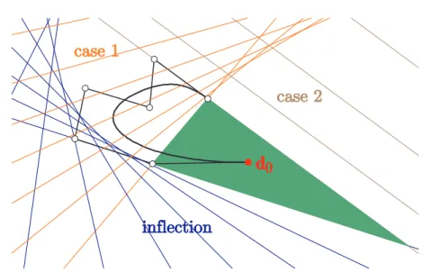
Figure 3: A convex Bézier curve with concave control polygon.
While control point d0 is in the green region the curve remains convex.
curve (2.3) becomes
l0(u) =− r0(1)−r0(u)
B0n(1)−B0n(u)= dn−r0(u) B0n(u)
and direction q0(u)is
q0(u) = (r0(u)−r0(1)) ˙Bn0(1) +˙r0(1) (B0n(1)−B0n(u))
=−nB0n(u) (dn−dn−1),
i.e. q0(u)is parallel to the directiondn−dn−1for any permissible value ofu. Fig.
3 illustrates the different regions that are used for the convexity test for a Bézier curve of degree 6.
References
[1] Farin, G., Curves and surfaces for CAGD: A practical guide, 4th ed., Academic Press, San Diego, 1999.
[2] Juhász, I., On the singularity of a class of parametric curves,Computer Aided Geo- metric Design, 23 (2006) 146–156.
[3] Liu, C., Traas, C. R., On convexity of planar curves and its application in CAGD, Computer Aided Geometric Design, 14 (1997) 653–669 .
[4] Pottmann, H., Wallner, J.,Computational line geometry, Springer-Verlag, Berlin, 2001.
[5] Prautzsch, H., Boehm, W., Paluszny, M., Bézier and B-spline techniques, Springer-Verlag, Berlin, 2002.
[6] Ralston, A., Rabinowitz, P., A first course in numerical analysis, 2nd ed., McGraw-Hill, New York, 1978.