in focus labour market effects of the crisis

LABOUR MARKET EFFECTS OF THE CRISIS

Edited by

György Molnár

PREFACE

The In Focus section of The Hungarian Labour Market usually examines one specific area of the labour market based on available Hungarian empirical re- search results. This time, we have expanded our perspective to a greater extent than usual, and have attempted to assess the effect of the crisis on the entire labour market, in fact including a survey of the effects on households as well.

Until now, the In Focus section has mostly presented well-developed research results that have been previously evaluated during academic debates. On the topic of the crisis, we cannot expect such a synthesis, since the processes un- der study have not yet reached completion and the longitudinal datasets nec- essary for the analysis are short, in actual fact, in the case of some topics (for example, household consumption), data covering the time period of the crisis are not yet available.

Despite these difficulties, more than two years after the beginning of the cri- sis, we must reflect on it in depth. An extraordinary situation demands unusual reactions in research and in publication as well. This is also why we feel that it is necessary to consider not only direct, short-term labour market effects, but also indirect, long-term processes that manifest themselves via the households and the reproduction of the workforce. The labour market phenomena of the crisis cannot be understood if we disregard the responses of firms and households.

In the first chapter of In Focus, János Köllő examines the evolution of em- ployment, unemployment, and wages in the first year of the crisis. The study focuses on the changes in the number of employees, average monthly paid work hours, and gross hourly incomes – and the relationship between these – based on calculations using a panel sample comprised of more than five thousand firms that were observed in May of both 2008 and 2009 in the wage survey of the National Employment and Social Office. The most important result of this analysis is that in the first year of the crisis, Hungarian firms mainly respond- ed to the fall in demand, the narrowing of loan opportunities, and the falter- ing of business confidence by downsizing employment. Based on data from the labour force survey of the Hungarian Central Statistical Office (HCSO), it can also be stated that the decrease in employment was primarily due to the deferred hiring of employees. The study concludes with a brief overview of the employment policy response to the crisis.

The In Focus section, in line with the practice that has evolved over previ- ous years, briefly touches on a few topics related to the more detailed analyses.

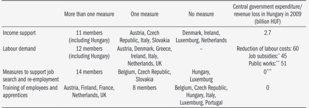
The study by Péter Elek and Ágota Scharle takes account of the European, and

within these, the Hungarian policy measures that were aimed at dampening the employment effects of the economic downturn. They find that the most important elements of Hungary’s crisis management were the encouragement and protection of labour demand.

András Semjén and János István Tóth provide a brief overview, based on firm survey data, of the steps taken by firms in response to the crisis. The results of the survey suggest that firms typically combine several different reactive measures that are effective in the short-term, and proactive crisis management measures that lead to long-term adaptation – no single preferred corporate strategy for crisis management can be pinpointed.

Compared to comprehensive analyses based on data reflecting the entire firm sector, Dorottya Boda and László Neumann use a different methodology. The authors summarize the results of two empirical studies, which mainly exam- ined the effect of the crisis on firm management based on firm interviews. The study shows, through telling examples, under which conditions, and as a result of which employment decisions, do the specific events that can be measured in the labour market evolve. During this analysis, they also make note of the symptoms of the crisis that are felt by firms, the crisis management measures that have employment effects, and the role of government supports and the representatives of employee interests.

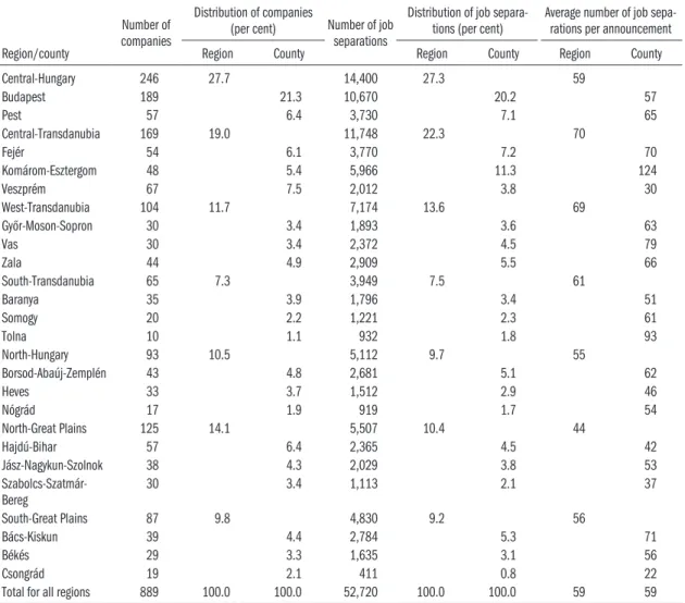
The data-rich study of Irén Busch and György Lázár demonstrates the main characteristics of an important subset of firm human resource measures, ma- jor layoffs. Comprehensive data regarding this area are available via mandatory reporting-based datasets of the Public Employment Service. After an introduc- tion of the legal background the authors compare the evolution of announced layoffs and registered unemployment over the last 10 years, then examine the developments between October of 2008 and June of 2010 in greater detail. The authors had the opportunity to link the data of workers affected by layoffs to the database of registered job seekers, so they were also able to track the evolu- tion of the labour market status of affected workers.

The study by Hajnalka Lőcsei analyzes the effect of the crisis on regional in- equalities in unemployment using the database of registered jobseekers. Based on the speed and type of the changes, she divides the time period between the fall of 2008 and the summer of 2010 into four sections, and describes the evolution of the spatial expansion of unemployment for each of these. She de- termines that during the first stage of the crisis, the number of job seekers in- creased significantly mostly in the districts with export-oriented firms, the most developed regions, and, within these, in the source locations of commuters.

Later on, however, increasing unemployment became a regionally generalized phenomenon. Up until the lowest point of the crisis, the spatial duality of the labour market lessened somewhat and regional differences decreased, but this effect will probably only be temporary.

The regional analysis is completed by two short studies. The study by Albert Faluvégi examines in more detail how the crisis affected the most disadvan- taged micro-regions. He demonstrates the procedure for selecting these areas as well as their main characteristics, of which the very high, more than double the national average, unemployment stands out. He shows that the unemploy- ment rate of these areas continued to increase during the crisis, but the devia- tion from the average decreased somewhat – mostly due to the expansion of public employment.

The issue of commuting is an important component of the evolution of em- ployment differences. Tamás Bartus analyses the relationship between com- muting time and the rural-urban wage difference. The data needed for the calculations of the model are only available for the time period prior to the transition, but these also provide some important implications. The most im- portant finding of the study is that in disadvantaged regions, the estimated costs due to time lost commuting reach and surpass the wage increases that can be achieved.

Due to the lack of recent data, the longer study of András Semjén and János István Tóth also attempts to draw conclusions based on earlier analyses regard- ing the effects of the crisis on unreported employment. Within unreported employment, they focus on two types: “under the table” payments and “billed payments”. Differentiating between 13 types, they review what kind of effects the crisis may have had on the ratios of reported and unreported employment, or employment concealed as entrepreneurial activity. Their conclusion is that the economic crisis probably led to unreported or concealed work spreading more widely, and increasing in volume over the last two years.

The effect of the crisis on households stands at the center of the following studies. The micro-simulation analysis of Katalin Gáspár and Áron Kiss exam- ines how the income position of households in different situations changed as a result of layoffs in the first year of the crisis. Using different characteristics from the labour force survey of the HCSO, they estimate the likelihood of job loss of employees and then analyze the income effects of job loss based on household budget surveys. Among other conclusions, they find that the prob- ability of job loss is two to three times higher in the case of employees in lower income groups compared to that observed in higher income groups. The ab- solute value of the average income loss due to job loss increases with income level, but the relative income loss is of similar magnitude for all income groups.

The study of István György Tóth and Márton Medgyesi is composed of two main parts. First, they demonstrate the long term evolution of the main indica- tors of the income distribution based on the Tárki household monitor survey, with a special focus on the changes between 2007 and 2009. These processes reflect not only the effects of the crisis, but also those of the consolidation meas- ures of the earlier years. They find that in the last period, the situation of both

the rich and the poor has deteriorated, but that of the poor worsened signifi- cantly. Compared to the “depolarization” observed earlier, the most important change is the polarization that occurred at the bottom of the income distribu- tion. When examining polarization in employment, they reach the conclusion that employment decreased most in the case of those groups that previously had two employed workers in their household. The second part of the study details subjective living difficulties, the indebtedness of households and their difficulties paying off their loans. The ratio of households that were in need and reporting financial difficulties increased between 2007 and 2009. Diffi- culties repaying debt increased, primarily in the case of lower income groups.

The brief study by Zsuzsa Kapitány is related to the latter topic and demon- strates the changing consumer behaviour of households in the real estate and mortgage market. The study discusses the effect of the crisis on households ac- quiring loans and specifically mortgage loans, the evolution of late payments, as well as the effects on the real estate market and real estate construction. She finds that households were forced to decrease their consumption sharply and to constrain acquiring loans, primarily mortgage loans, significantly as a result of the crisis, so the household sector as a whole became a net loan re-payer. At the same time, the ratio of those who made late payments or missed payments increased significantly.

Due to the unique nature of this year’s In Focus, we felt it necessary to include a non-traditional summary at the end of the section, which was prepared by the editor, György Molnár. In this, we aim to provide an overall picture of the most important results of the studies in the In Focus section, highlighting the relationships between the different studies as well as the differences that arise from the different approaches used by their authors.

1. EMPLOYMENT, UNEMPLOYMENT AND WAGES IN THE FIRST YEAR OF THE CRISIS^*

János Köllő Introduction

In 2009, the average annual stock of employed persons fell by about one hun- dred thousand compared to 2008. In relative terms, the number of employees was cut by 3.6 or 3.7 per cent, depending on how employee status is defined, while ILO-OECD employment decreased by 2.5 per cent, as shown in Table 1.1.¹

Table 1.1: The number of employed persons and employees in 2006–2009 (thousands)

Year

Employed

Employees

Average annual number of persons participating in the activity of eco-

nomic organizations Population aged

15–64 Population aged 15–74

2006 3,906 3,930 2,790 2,829

2007 3,897 3,926 2,761 2,806

2008 3,849 3,879 2,762 2,812

2009 3,751 3,781 2,661 2,710

Change 2009/2008

Thousand –98 –98 –101 –102

Per cent –2.5 –2.5 –3.7 –3.6

Source: Website of the Hungarian Central Statistical Office (http://ksh.hu). The first two columns are based on the Labour Force Survey while columns 3 and 4 are establishment-based.

Employment measured in hours fell by a slightly higher rate because the aver- age monthly working hours of employees diminished by a little more than one per cent, as will be discussed later in more detail.

The ILO-OECD unemployment rate of prime age males (15–61 year olds) jumped from 7.8 per cent in July-December 2008 to 10.0 per cent in January- June 2009 while the respective figures were 8.1 and 9.4 per cent for women.² Alternative indicators of unemployment followed similar time paths as shown in Table 1.2, and continued to grow until the first quarter of 2010. At the peak, in January-March 2010, the ILO-OECD rate reached 11.9 per cent, a level un- precedented since 1995.³

The growth of unemployment was accompanied by a decline of the real wage.

In 2009 the gross real wage fell by 3.4 per cent and the net real wage de creased by 2.3 per cent.⁴

* This chapter draws heavily from a study commissioned and published by the ILO and forth- coming at Edward Elgar (Köllő 2011). It also includes translated excerpts from Köllő (2010).

1 According to the ILO-OECD definition, a person is employed if she/he did at least one hour of gainful work in the week pre- ceding the interview, or, was only temporarily absent from an existing job.

2 The data come from the Labour Force Survey, where individuals (i) out of work, (ii) ready to take up employment and (iii) actively searching for jobs are classified as unemployed, following the guidelines of the ILO and the OECD.

3 http://portal.ksh.hu/pls/

ksh/docs/hun/xftp/gyor/fog/

fog21003.pdf.

4 According to the HCSO’s on- line Stadat data base (August 26, 2010) gross and net earnings increased by 0,6 and 1.8 per cent while consumer prices went up by 4.2 per cent.

Table 1.2: Unemployment rates^a using alternative definitions of joblessness Definitions

of unemployment

2006 2007 2008 2009

I. II. I. II. I. II. I. II.

Male

– Actively searching 7.3 7.2 7.2 7.2 7.6 7.8 10.0 10.8

– Registered 7.6 7.2 7.4 7.3 8.3 8.3 10.1 10.5

– Would like to work^b 12.5 11.8 12.0 11.8 12.6 12.6 15.1 15.7 Female

– Actively searching 7.7 8.1 7.4 8.0 8.2 8.1 9.4 10.2

– Registered 8.8 8.9 8.6 8.4 8.9 8.9 10.2 10.9

– Would like to work^b 15.1 15.1 14.5 14.5 15.2 15.0 16.6 17.2

a The unemployment rate is calculated as U/(E + U), where E is employment according to the ILO–OECD definition and U is the number of unemployed according to the definition given in the respective row

b Is not actively searching but wants paid employment Note: The data relate to persons aged 15–61.

Source: Labour Force Surveys, author’s calculations.

The most comprehensive international comparative survey of reactions to the crisis so far (Verick–Islam, 2010) ranks Hungary among countries including Finland, Croatia and Slovenia, where a substantial fall of GDP was associated with a moderate fall of employment. The paper also examined the role of work- ing time adjustment within total employment adjustment in the manufactur- ing industry. In this respect, Hungary, Croatia and The Netherlands form a triad characterized by a substantial fall in the number of employees and mi- nor cuts of working hours. Counter-examples are Germany, Austria, Island and Malta, where shortening the workweek made a decisive contribution. In Ireland, Estonia and Slovakia working time reductions played a less prevalent but still important role.

For the time being, there are several obstacles hindering a reliable cross-coun- try comparison. Data on real wage evolutions during the crisis are still missing in several countries and time series distinguishing the public and private sec- tors are hardly available. The existing figures on wages and working time typi- cally relate to the manufacturing industry while the data on employment and GDP cover the whole economy. For the moment, only the latter indicators can be used for meaningful international comparison.

Panels a and b of Figure 1.1 show the position of OECD member states (and some other European countries) in terms of changes of GDP and employment in 2009. The best-fitting regression lines are added. The output elasticity of employment (slope of the regression line) is 0.62 for all countries and 0.42 for countries excluding the Baltic states, which experienced an extreme, two-digit fall in their GDP. The respective indicator (log change of employment divided by log change of GDP) amounted to 0.35 in Hungary. Even though employ- ment fell mildly relative to the fall of GDP, Hungary ranks among the big los-

ers of the crisis in terms of absolute change of employment: the vast majority of OECD countries (23 out of 35 shown in Figure 1.1) performed better in terms of employment change than did Hungary.

–1.5 –1.0 –0.5 0.0 0.5

–0.2 –0.15 –0.1 –0.05 0.0 0.05

GDP 2009/2008 (log)

Employment 2009/2008 (log)

–0.1 –0.05 –0 0.05

–0.08 –0.06 –0.04 –0.02 0 0.02

GDP 2009/2008 (log)

PL KORAUS CH TRLUX

MEX D A B

GRF CDNP USA

IS E

NZ NCHI

LV

EST LT

IRL SF

RO H DKSK

BG CZNL SVGB I

Estimated value

AUS PL TR

LUX

D B F

IS

CZNL SVI GB PL

KORAUS CH TRLUX

MEX D A B

GRF CDNP USA

IS E

NZ NCHI

LV

EST LT

IRL SF

RO H DKSK

BG CZNL SVGB

I KOR

MEX CH

A CDN GR

P USA

E

NZ N CHI

IRL SF

RO H

DK BG SK

Figure 1.1: Changes of GDP and employment in 36 countries, 2008–2009

a) All countries b) Without Baltic states

Abbreviations: A – Austria, AUS – Australia, B – Belgium, BG – Bulgaria, CDN – Canada, CH – Switzerland, CHI – Chile, CZ – Czech Republic, D – Germany, DK – Denmark, E – Spain, EST – Estonia, F – France, GB – United Kingdom, GR – Greece, HU – Hungary, I – Italy, IRL – Ireland, IS – Island, KOR – Korea, LT – Lithuania, LUX – Luxemburg, LV – Latvia, MEX – Mexico, N – Norway, NL – Netherlands, NZ – New Zealand, P – Portugal, PL – Poland, RO – Romania, S – Sweden, SF – Finland, SI, – Slo- venia, SK – Slovakia, TR – Turkey, USA – United States. Source: OECD and Eurostat on-line data bases, August 12, 2010

Figures similar to the ones presented in Figure 1.1 are to be interpreted with caution since they merge the public and private sectors, which followed rather different paths in many countries, including Hungary. The means relating to the whole economy are hotchpotch indicators that actually do not reflect the underlying processes taking place in either parts of the economy. As shown in Table 1.3, employment grew in the public sector while the real wage fell by two-digit percentages. By contrast, in the private sector, the real wage remained virtually unchanged and employment was cut substantially by 6.7 per cent.

Table 1.3: Changes of employment, wages and working hours, 2009 Public sector^a Private sector^b Total

Number of employees 3.6 –6.7 –3.7

Real gross monthly earnings^c –11.6 0.1 –4.5

Average monthly working hours per employee^d –1.3 –1.1 –1.1

a Nonprofits included. Employees include those doing public works.

b Firms employing at least 5 workers.

c Consumer price index: 1.042.

d Annual mean of quarterly figures.

Source: HCSO Stadat, August 25, 2010 except for working time: June 8, 2010.

In the remainder of this chapter we study the dynamics and relation to each other of changes in employment, wages and working hours in the private sec- tor. It seems that there is no point in repeating the analysis for the public sec- tor, where the number of permanent employees did not change (fell by 0.4 per cent excluding people doing public works) and wages fell as a result of across- the-board measures such as the abolishment of the 13^th month’s salary and an (unofficial but effective) ban on pay rises. Therefore, in the public sector, we do not expect remarkable structural changes to be explained.

The study of the private sector is primarily concerned with the issue of “hard”

versus “soft” adjustment. The countries of Europe reacted to the crisis in sharply different ways: in Germany, unemployment grew by 0.2 percentage points de- spite a 5 per cent fall of GDP while in Spain a recession implying a 3.6 per cent fall of GDP brought about a 6.7 percentage points increase in unemployment (Verick–Islam, 2010, 25). In Hungary, there was much talk about soft adjust- ment via shortening the workweek and pay cuts, but the actual contribution of these measures should be judged on the basis of data rather than media coverage.

Soft versus hard adjustment

In a competitive labour market with finitely elastic supply and demand, both employment and wages are expected to respond to a negative aggregate shock.

Why the textbook predictions so often fail is an old and much debated ques- tion in labour economics. Several theories have been developed to understand why we observed large fluctuations in employment, and small ones in the real wage, over the business cycles of the US and some other developed market economies. In a monopoly union setting or in the case of efficient bargaining, for instance, we expect that the burden of adjustment predominantly falls on employment (McDonald and Solow 1982, Brueckner 2001). Similar conclu- sions follow from the theories of implicit contracts (Azariadis 1975, Feldstein 1976, 1978, Rosen 1985) and intertemporal substitution over the life cycle (Lucas and Rapping 1969).

Despite the theoretical predictions of strong cyclicality in employment and less in wages the recent empirical evidence is mixed. In a study of the cyclical- ity of manufacturing employment and wages between 1960 and 2004 Messi- na, Strozzi and Turunen (2009) find substantial cross-country variations even after controlling for the type of data and methods used in measuring cyclical- ity. They identify positive correlation between the cyclicality of real wages and the cyclicality of employment, but identify groups of countries having rather different positions along these dimensions. The available data on the current crisis also suggest high diversity across countries.

In a transitory downturn, reductions in hours and pay cuts may be attractive options if firing and hiring costs are high and firm-specific skills are impor- tant. When plant utilization is temporarily low, firms may also prefer training

their workers since the costs of accumulating firm-specific skills are lower. Re- acting to a negative shock in ways other than dismissals is easier if institutions supporting the adjustment of hours and wages are at hand, as emphasized in Bellmann and Gerner (2009). One institution of this kind is working time ac- counts allowing that employees work longer or shorter hours than usual and thereby collect working time credits or debits in an individual account, which are later compensated for by additional leisure or work. Similarly, softer meas- ures can be encouraged by pacts for employment and competitiveness in which employees accept lower wages and reduced working time and employers guar- antee jobs, training, and offer financial participation (Bellmann, Gerlach and Meyer 2008). Profit sharing can also make wage adjustment easier since it es- tablishes an automatic link between workers’ pay and the fluctuations of busi- ness fortune.

The institutional features of the Hungarian labour market make the adjust- ment of both employment and wages relatively easy but there are few formal agreements and legal institutions explicitly encouraging a heterodox reaction to a negative shock.

Union coverage is low and has been declining since the start of the transition.

According to the Labour Force Survey, the share of union members amounted to 20 per cent in 2001, 17 per cent in 2004 and 12 per cent in 2009. The pro- portion of workers employed in unionized firms fell from 38 per cent in 2001 to 33 percent in 2004 and 28 per cent in 2008. The share of workers covered by collective agreements declined from 25 per cent in 2004 to 21 per cent in 2009. The agreements are typically concluded with a single-employer and are not extended. Furthermore, the unions seem to be relatively weak as suggest- ed by estimates of a small (0–2 per cent) regression-adjusted union wage gap (Neumann 2002, Rigó 2009).

There are few legal constraints on employment and wage setting, with the most important one being the minimum wage. The minimum wage-average wage ratio (34.7 per cent just before the crisis) can not be considered high by inter- national comparison but the real minimum wage has been constantly grow- ing over the last ten years. The adjustment of the minimum wage is negotiated annually at the national level, by employer organizations and unions, allowing careful policies in hard times, but unions generally start the negotiations with ambitious goals and usually achieve at least modest increases in real terms.⁵ It was the case at the beginning of the recent crisis too, as will be discussed later.

Only a single estimate of adjustment costs is available (Kőrösi and Surányi 2003) suggesting that hiring and firing are relatively inexpensive by interna- tional comparison. Training costs probably do not play an important role in firms’ decisions since the fraction of Hungarians participating in adult train- ing is one of the lowest in Europe and on-the-job training is particularly in- frequent (Bajnai et al. 2009). Hungary’s employment protection (EPL) index

5 The real net minimum wage increased in all years between 1998 and 2008.

is the lowest in Central and Eastern Europe and one of the lowest in the EU (Cazes and Nesporova 2007).

Institutions encouraging the combination of employment, hours and wage adjustment are undeveloped in Hungary. Formal agreements similar to the pacts for employment and competitiveness do not exist to the best of the au- thor’s knowledge. Working time accounts have not been established as a le- gal institution, in contrast to the Czech Republic and Germany, for instance, where about half of the medium-sized and large companies are covered (Bell- mann and Gerner 2009). The fraction of workers involved in profit sharing agreements is one of the lowest in Europe with Hungary preceding only Por- tugal and Cyprus (European Foundation 2007). Still, it would be mistaken to rush to the conclusion that these practices simply do not exist. We have ample anecdotal evidence that working time accounts are applied informally. Profit sharing also exists informally as suggested by a relatively high elasticity of wag- es with respect to the firm’s productivity (Mickiewicz and Köllő 2004, Com- mander and Faggio 2004). Employer and employees may also conclude infor- mal agreements on saving jobs by means of soft measures, and we hope to find the traces of such agreements when we look at how firms actually combined staff reductions, wage cuts and reductions in hours during the current crisis.

Firms’ reactions to the crisis

In this section, we look at variations in the changes of employment, hours and wages using longitudinal firm-level data covering May 2008 and 2009. The estimation of a full causal model – explaining how the crisis affected firms’

decisions on the level and composition of employment and wages – is beyond the capacity of the data at hand. We do not have, as yet, firm-level data on the changes of output and other variables capturing the size of the shock to which the firm had to respond. This will be approximated with two-digit industry- level data on the changes of output, which is an admittedly second-best solu- tion. Equally important, the identification of causal effects in a system with several endogenous variables would require exogenous instruments having impact on particular outcomes without affecting others. Such instruments are not available in the data set. The available variables like firm size, industry, ownership, union coverage, exposure to the minimum wage and skill compo- sition are likely to affect employment, hours and wages simultaneously. There- fore we use a descriptive three-equations model explaining the log change of employment (L), monthly working hours (H) and average hourly wages (w) .

ΔlnL_i = Xiβ + u_i (1a)

ΔlnHi = Xiγ + vi (1b)

Δlnw_i = Xiδ + ω_i (1c)

The equations have the same set of explanatory variables (X) so the coeffi- cients and the standard errors are the same as if the equations were estimated one by one with OLS. By estimating (1a-1c) jointly as a system of seemingly unrelated regressions we can study the correlations between the residuals u, v and ω and test if the three equations are independent.

In a second step, we show that the changes of average wages were strongly affected by changes in the firms’ skill composition. By regressing Δlnw– on changes in the demographic and skill composition of the workforce and tak- ing the residuals (ζ) as in equation (2) we can get a measure that is controlled for compositional effects. (In the equation AGE stands for average age, EDU denotes average years in school and MALE relates to the share of men within the firm.) Then, after replacing Δlnw– with ζ in an equation similar to (1c), we can check how residual wages were affected by the X-s.

ζi = Δlnw–i – β1ΔAGEi – β2ΔEDUi – β3ΔMALEi– c. (2) The analysis relates to 5,173 firms observed in 2008 and 2009 in the Wage Survey (WS). A description of the survey, analysis of selection to the panel and a comparison of descriptive statistics to published figures are presented in Appendix 1. Here we turn to the estimation results presented in Table 1.4.

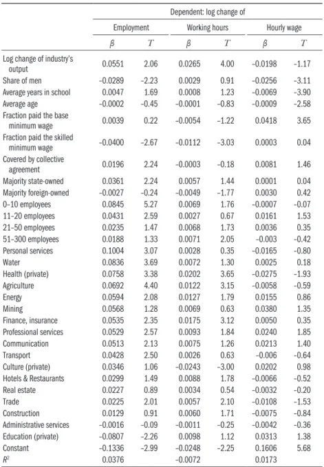
As shown in the first row, industry output has a significant positive effect on both employment and hours and has no effect on wages. The estimated elas- ticity is rather weak (0.055) and most probably downward-biased since the in- dustry’s change of output measures the firm-specific shocks with a wide mar- gin of error. Unfortunately, firm-level data and three or four-digit sector level data were not available at the writing of this text. The change in output had a weak effect on working hours (0.027) and no effect on wages.

Male-dominated firms lost more jobs and had worse-than-average wage re- cords. Firms, in which the male’s share was higher by one standard deviation (31 per cent) lost more by about 1 per cent in terms of employment and 0.7 per cent in terms of average wages. Skills also seem to matter: a one standard de- viation (1.5 year) difference in workers’ average years in school implied about 1 per cent higher employment and 1.1 per cent lower wage in 2009 relative to 2008. Average age had no effect on employment and hours but affected wages marginally: a workforce older by 6.3 years (one standard deviation) implied that wages grew slower by 0.6 per cent.

Firm size has a marked effect on employment and some impact on hours while its effect on wages is insignificant. Small and medium-sized firms lost less jobs than large ones (300+ employees) by 8, 4, 2 and 2 per cent, respectively, as we move from the bottom to the top of the size ladder. This pattern is probably explained by differences in exposure to exports: we find the advantage of the smallest firms to be much larger (12 per cent) in manufacturing, where larger firms tend to be either exporters or suppliers of exporters, than in the rest of the economy (5 per cent).

Table 1.4: Changes of employment, working hours and hourly wages – multivariate regressions (firm panel)

Dependent: log change of

Employment Working hours Hourly wage

β T β T β T

Log change of industry’s

output 0.0551 2.06 0.0265 4.00 –0.0198 –1.17

Share of men –0.0289 –2.23 0.0029 0.91 –0.0256 –3.11

Average years in school 0.0047 1.69 0.0008 1.23 –0.0069 –3.90

Average age –0.0002 –0.45 –0.0001 –0.83 –0.0009 –2.58

Fraction paid the base

minimum wage 0.0039 0.22 –0.0054 –1.22 0.0418 3.65

Fraction paid the skilled

minimum wage –0.0400 –2.67 –0.0112 –3.03 0.0003 0.04

Covered by collective

agreement 0.0196 2.24 –0.0003 –0.18 0.0081 1.46

Majority state-owned 0.0361 2.24 0.0057 1.44 0.0001 0.04

Majority foreign-owned –0.0027 –0.24 –0.0049 –1.77 0.0030 0.42

0–10 employees 0.0845 5.27 0.0069 1.76 –0.0007 –0.07

11–20 employees 0.0431 2.59 0.0027 0.67 0.0161 1.53

21–50 employees 0.0235 1.47 0.0068 1.73 0.0036 0.35

51–300 employees 0.0188 1.33 0.0071 2.05 –0.003 –0.42

Personal services 0.1004 3.07 0.0028 0.35 –0.0165 –0.80

Water 0.0836 3.69 0.0072 1.30 0.0025 0.18

Health (private) 0.0758 3.38 0.0202 3.65 –0.0275 –1.93

Agriculture 0.0692 4.40 0.0122 3.15 –0.0058 –0.59

Energy 0.0594 2.08 0.0127 1.79 0.0155 0.86

Mining 0.0568 1.28 0.0069 0.63 0.0380 1.35

Finance, insurance 0.0535 2.35 0.0175 3.12 0.0050 0.35

Professional services 0.0529 2.57 0.0093 1.84 0.0240 1.85

Communication 0.0513 2.13 0.0075 1.26 0.0213 1.40

Transport 0.0428 2.50 0.0026 0.63 –0.006 –0.64

Culture (private) 0.0346 1.06 –0.0243 –3.00 0.0202 0.98

Hotels & Restaurants 0.0299 1.49 0.0088 1.78 –0.0066 –0.52

Real estate 0.0227 0.89 0.0034 0.54 –0.0032 –0.20

Trade 0.0225 2.01 0.0057 2.10 –0.0108 –1.53

Construction 0.0129 0.91 0.0060 1.71 –0.0075 –0.84

Administrative services –0.0016 –0.09 –0.0011 –0.25 –0.0042 –0.36

Education (private) –0.0807 –2.26 0.0098 1.12 0.0313 1.38

Constant –0.1336 –2.99 –0.0248 –2.25 0.1606 5.68

R² 0.0376 –0.0072 0.0173

Correlation of the residuals:

Employment-hours: 0.0117. Employment-wage: –0.0072. Hours-wage: –0.3107 Breusch-Pagan test of independence: chi2=500.185 (0.0000)

Number of observations: 5,173

Reference industry: manufacturing. Industries are ordered by the size of the coeffi- cients in the employment equation.

As far as industry effects are concerned, the employment records of manufac- turing, construction and real estate appear to be statistically identical, while retail trade, hotels and restaurants seem to have lost fewer jobs. Three groups of sectors stand out (i) water, energy and transport (ii) personal services, finance and insurance and (iii) agriculture. In these sectors, employment fell less by 5–9 per cent relative to manufacturing (where it was cut by 12.2 per cent) even after controlling for the change in sales revenues. Inelastic domestic demand for some of the aforementioned services, market power and a high share of self-governing firms (family businesses, partnerships of friends and relatives) are factors potentially explaining why employment suffered less in these in- dustries. We do not observe trade-offs between employment and hours and/

or wages on the sector level: in sectors losing less jobs average working hours changed favorably, too, while the industry wage effects were insignificant with only two exceptions (agriculture and professional services, both weakly signifi- cant at the 5 per cent level).

State-owned firms lost fewer jobs than did domestic private ones by 3.6 per- cent, and held average hours higher by 0.6 percent. In terms of wages they did not differ from their private counterparts. The estimates relating to foreign firms are insignificant and hint at negligible difference between them and do- mestic private enterprises.

Exposure to changes in the minimum wage is measured with the fraction earning near the base minimum wage (MW±1,000 HUF) and the skilled minimum wage (SMW±1,000 HUF). More workers paid the MW in the base period predict faster average wage growth but having more SMW earners has no wage effect. A firm with only MW earners increased the average wage faster by about 4 per cent compared to a company with no MW earners, consistent with the fact that the base MW grew by 3.6 per cent. At the same time, we do not observe larger-than-average employment and hours cuts in firms with more MW earners. Firms with many SMW workers did lose more jobs and also cut working hours more than did their observationally similar counterparts. These cuts are hardly explained by the tiny (0.8 per cent) rise in the nominal SMW but the existence of a floor may have prevented enterprises from reducing the wages of skilled employees.⁶

Finally, the estimates suggest that firms covered by collective agreements valid for 2009 kept the level of employment higher by about 2 per cent compared to their observationally similar counterparts. The estimates relating to working hours are insignificant. It seems that wages grew slightly faster than elsewhere but the coefficients are not significant at conventional levels.

To summarize the regression results, the employment effects of the variables in equation (1) are mostly significant and often rather strong. The variations in average working hours seem much smaller while wage evolutions were large- ly unrelated to the variables in the model. Apart from the variables depicting

6 In 2008 the regulations dis- tinguished three mandatory minima: the base minimum wage (MW), the skilled mini- mum wage (SMW=1.25MW) and a reduced minimum for younger skilled workers with less than 3 years experience (YSMW=1.2MW). In Septem- ber 2008, the unions started the negotiations with the claim of a 15.9 per cent rise in the MW, 14.7 per cent rise in the YSMW and 10.1 per cent rise in the SMW starting from January 2009.

Given a consensus inflation forecast of 4.2 per cent at the start of the negotiations these hikes would have implied 11.2, 10.0 and 6.3 per cent increase of the minima in real terms, respectively. Even at the end of November, two months into the crisis, the unions demanded a 10.9 per cent rise in the base MW in nominal terms, and insisted on their original claims regard- ing the SMWs. Finally, under the pressure of the crisis the parties agreed to a 3.6 per cent increase of the MW, 5.1 per cent rise in the YSMW and a mere 0.8 per cent rise in the SMW in nominal terms. More precisely, the negotiations resulted in the elimination of YSMW and the setting of a uniform SMW equal to 87,000 HUF, which implied the percentage changes quoted above.

the base-period composition of the workforce and the share of MW earners almost all the other variables in equation (1c) are statistically insignificant.

The only significant variable in the wage equation re-estimated with ζ rather than Δlnw– on the left hand is the base-period share of MW earners. (The coef- ficient is 0.053, significant at the 1 per cent level.) Since ζ captures the change in the cost of labour more precisely than Δlnw– we conclude that wage evolutions were unrelated to industry, firm size, ownership, union coverage and region.⁷ On closer inspection the same seems to apply to the effect of skill composition.

The employment and wage equations (1a, 1c) give the impression that firms with a skilled labour force adapted to the crisis by cutting wages but keeping employ- ment relatively high – an outcome consistent with expectations grounded in the theories of quasi-fixed costs and firm-specific skills. The re-estimated equa- tion suggests that the cost of labour actually did not fall in these enterprises – this is a statistical illusion generated by the changing composition of the staff.

Firms employing many skilled workers dismissed more skilled workers, even in relative terms, which led to lower average wages.

The close-to-zero correlations between the residuals u, v and ω of equations (1a-1c) suggest that the firm-specific changes of employment and hours, and employment and hourly wages, were independent of each other. By contrast, the residual changes of hours and hourly wages are relatively strongly correlat- ed (–0.31). This result arises for two reasons. On the one hand, monthly earn- ings do not fall proportionately when working hours are cut therefore falling hours are associated with rising hourly earnings. On the other hand, errors in the reporting of hours can establish a spurious correlation between Δw and ΔH.⁸ In view of this risk, a system similar to (1a-1c) was estimated by dropping the hours equation and working with monthly rather than hourly wages. The residual correlation between the changes of employment and monthly wages amounted to –0.02 in this case, too, and the Breusch-Pagan test did not reject the independence of the two equations.

A note on union effects

The finding that employment fell less in unionized firms as in the rest of the private sector, all else equal, is an interesting one but needs further inspection.

The OLS results can be biased for at least two reasons.

First, controlling the employment equation for firm size, industry and other variables is insufficient to ensure that we compare comparable firms. Therefore the employment effect of collective agreements is further analyzed with pro- pensity score matching following Rosenbaum and Rubin (1983). We use Stata’s pscore module developed by Becker and Ichino (2002) at this aim. As shown in Table 1.5 nearest neighbor matching suggests a statistically insignificant effect of 1.7 per cent while the stratification method and the kernel matching model results in significant effects of 1.9 and 2.0 per cent, respectively.⁹

7 The regional variables (NUTS- 3 dummies, NUTS-4 unemploy- ment rates) were insignificant in all specifications and dropped from the models.

8 Assume that all firms cut work- ing hours but only some of them report it. Assume further that all firms hold genuine hourly wages constant. In the non-reporting group, the estimated hourly wages (monthly pay/observed hours) fall and observed hours remain constant. In the report- ing group the calculated hourly wage rises and observed hours fall. At the end of the day we observe a negative correlation between the observed changes of hours and hourly wages.

9 Note that the estimated effects are “average treatment effects on the treated” (ATT), larger than the average treatment ef- fects (ATE) capturing the re- turns to coverage for a randomly selected firm.

Table 1.5: Estimates of the effect of collective agreements on the changes of employment 2008–2009

Model Effect t

OLS 2.0^*** 2.24

ATT nearest neighbor matching^b 1.7 1.44

ATT stratification method 2.0^*** 2.77

ATT kernel matching method 1.9^*** 2.26^c

a The propensity score equation included firm size, size squared and size cubed, share of men, average age and average years in school.

b The propensity score models were estimated for unweighted sample and excluding heavy outliers. ATT stands for average treatment effect on the treated.

c Based on bootstrapped standard errors with 200 replications.

Second, selection to treatment (having a collective agreement in 2009) might be affected by unobserved characteristics simultaneously affecting the prob- ability of concluding a collective agreement and the change of employment in 2009. It may be the case, for instance, that firms with a better outlook for 2009 were more likely to conclude an agreement with their unions or workers’

councils – in this case their favorable employment records should be interpret- ed as a cause rather than an effect. For addressing endogeneity we would need instruments correlated with coverage but uncorrelated with unobserved fac- tors implying better employment outcomes in 2009. Such instruments are not available in the WS data set. Therefore, we address endogeneity in an indirect way, by showing that firms foreseeing a larger decline in their industry’s sales revenues were more likely to conclude an agreement in 2009. Likewise, firms operating in high-unemployment regions were more likely to extend their col- lective agreements to 2009.

Table 1.6: The effects of industry-level change of output and local unemployment on the probability of being covered by collective agreement in 2009 (firm panel)

Sample

Number

of firms Covered in 2009

Logit^a marginal effect of industrial output May

2009/May 2008 (log) micro-region unemploy- ment rate 2007 (log)

All firms 5,432 1,480 –0.5745^***

(8.72) 00316^***

(3.25) Firms covered in 2008 1,407 1,067 –0.4694^***

(4.01) 0.0685^***

(3.70)

Firms uncovered in 2008 4,025 413 –0.5849

(1.02) 0.0295

(0.35)

a Logit with a coverage dummy on the left hand and the two listed variables on the right-hand.

Results from our substitute for the study of endogeneity are presented in Table 1.6. The first column shows that a one per cent difference in the industry’s out- put had a half per cent effect on the probability of concluding an agreement.

This result holds for all firms as well as firms having an agreement in 2008. The second column suggests that companies operating in high-unemployment re- gions were more likely to conclude a collective agreement in 2009. The coeffi- cients are similarly signed and have similar magnitudes in the case of firms un- covered in 2008 but covered in 2009, but the effects are statistically insignificant.

The data suggest that collective agreements were stimulated by hardships rather than expected improvements in the firm’s environment and call into question if the gains estimated with OLS and propensity score matching are illusory.

While the presence of unions was conducive to smaller than average rate of job loss, it did not imply that wages and working hours fell more than elsewhere.

The question of how profits and prices were affected remains a question to be addressed when financial data become available.

Rigidity of wages and working hours – further inspection using individual data

In evaluating the results presented in the previous section one has to consider that firm-level average wages and working hours had been calculated by aggre- gating individual data. The firm-level means are precise in the case of small firms (since the WS covers all of their employees) and sufficiently precise in the case of large firms (where the within-firm samples are large enough). However, in the case of medium-sized firms we generate the firm-level means using a small number of observations. The resulting measurement error leads to attenuation bias and leads to potentially mistaken conclusions concerning the impacts of firm-level attributes on wages and hours. In this section we study individual panel data, which confirm the conclusions drawn from the regression model in that they show the distribution of wages and working hours remarkably stable in 2008–2009. (See Appendix 1 on how the individual panel was constructed.) Wages

The four panels of Figure 1.2 show average wages in 2008 and 2009 in 100 per- centile groups of the 2008 wage distribution. Members of the panel were sorted by their earnings in 2008 and were divided into 100 groups. The base-period average earnings of these groups are measured on the horizontal axis while their earnings in 2009 are shown on the vertical axis. Base period earnings are also indicated on the vertical axis by a 45^o line. The closer a point to the 45^o line the smaller the change in the wages of the respective group. Panels a and b re- late to gross earnings while panel c and d show net figures. Wages in 2009 are expressed in real terms by discounting their values using the consumer price index (1.036 between May 2008 and 2009). In order to improve visibility the charts covering percentiles 1–75 and 76–100 are shown separately and loga- rithmic scales are applied. In chart a) the base minimum wage and the skilled minimum wage are indicated by vertical lines.

The charts suggest that real wages did not change in the middle and top of the distribution: in percentiles 12–100 the monthly gross real wage fell by 0.4 per cent while the net real wage grew by 1 per cent. By contrast, in percentiles 1–11 the gross and net real wage increased by 6.9 and 6.6 per cent, respectively.

Developments in this part of the distribution can not be explained by changes in the minimum wages since the base minimum wage did not change in real terms in 2009 and the skilled minimum wage actually decreased. Composi- tional effects can be ruled out as we compare groups of fixed membership. The observation is probably explained by random events: workers, who earned much less than their permanent wage in 2008 – for reasons of unpaid leave, sickness, or entry to the firm during May 2008 – returned to (or reached) their “normal”

wage level in 2009. The conjecture that large increases at the bottom of the dis- tribution are explained by such exceptional events is supported by the fact that median earnings did not rise in real terms in percentiles 1–11.

11.0 11.5 12.0 12.5

12.5 12

11.5 11

11.0 11.5 12.0

12 11.5

11

12.5 13.0 13.5 14.0 14.5

14.0 13.5

13.0

12.5 14.5

13.0 13.5 14.0

12.5

13.5 13.0

12.0 12.5

2008 2009

Figure 1.2: Individual earnings in 2008 and 2009 a) Gross earnings in percentiles 1–75

of the 2008 wage distribution b) Net earnings in percentiles 1–75 of the 2008 wage distribution

c) Gross earnings in percentiles 76–100

of the 2008 wage distribution d) Net earnings in percentiles 1–75 of the 2008 wage distribution

The individual data thus suggest that the insignificant, close-to-zero coeffi- cients estimated in the wage regressions are explained by the stability of the wage distribution rather than measurement error. In the first year of the crisis Hungarian firms left wages virtually unchanged. Changes in enterprise aver- age wages did occur but were unrelated to industrial and regional affiliation, firm size, ownership, union coverage and composition of the workforce.

Working time

Similar to the case of wages, our attempts at explaining the changes in work- ing hours might have failed because of measurement error. Therefore, in this section we check how paid working hours changed on the individual level be- tween May 2008 and 2009.

In the individual panel, the number of monthly paid working hours per em- ployee decreased by 1.6 per cent. The distribution of the 52,409 observed work- ers by change of working hours is shown in Figure 1.3. Panel a covers the cases falling to the range of ±60 hours per month. (Only 1.5 per cent of all workers fell outside this range). In order to improve visibility we add panel b that is re- stricted to changes in the ±40 hours range, and ignores zero change account- ing for more than 50 per cent of all observations.

Figure 1.3: The size distribution of members of the worker panel by change in their monthly paid working hours between May 2008 and 2009

a) Distribution in the range of ±60 hours b) Distribution in the range of ±40 hours. Zero change excluded

In both the positive and negative domains changes amounting to 8, 16, 24, 32 and 40 hours a month (1, 2, …, 5 days) occurred frequently and the columns indicating decreases are taller than those standing for increases. The difference is sizeable at 8 hours: people observing 8 hours fall in their monthly working time clearly outnumbered those having 8 hours increase. We conclude from these data that about 5 per cent of the total sample was affected by a typically minor shortening of working time.

Given that everybody working less than 40 hours a week is regarded as a part- timer in Hungary, the small change in working hours brought about a rela- tively large (5.5 percentage points) hike in the share of part-timers, as shown in the first row of Table 1.7. Further rows of the table help clarify how to eval- uate this figure.

First, there is a striking difference between the data reported by firms and workers: the number of LFS respondents reporting less than 40 hours of gain- ful work in the reference week (second row) grew only by 1.3 per cent. This gap is probably explained by the working of a “4 days work + 1 day training” pro- gram that was subsidized using EU funds. The program required that firms classify the involved workers as part-timers for the duration of the program while workers probably interpreted their obligation to attend training as work.

Table 1.7: Changes in different measures of part-time employment, 2008–2009 (percentage points)

Concept Data source Respondents Change

Actual paid hours in May fell short of 168 hours/month Wage Survey Firms 5.5 Actual hours in the reference week fell short of 40 hours LFS^b Workers 1.3

Had part-time contract in May HCSO ELS^a Firms 1.7

Had part-time contract in April-June LFS^b Workers 1.2

a Hungarian Central Statistical Office Establishment-based Labour Statistics 2008,

b Labour Force Survey, April-June, 2008, 20092009

Secondly, it seems that the workweek was often shortened without re-writing the worker’s employment contract: the share of such contracts grew only by 1.7 and 1.2 per cent according to firms and workers, respectively.

Altogether we perceive that relatively few people were shifted from full-time to part-time jobs in the first year of the crisis, even less on a permanent basis, and even the seemingly large changes (as the 5.5 per cent figure in the first row of Table 1.5) hide small shifts in actual working hours. Predictably, a large part of these changes were accounted for by government-sponsored programs. Ac- cording to establishment-based statistics¹⁰ the number of part-time employees in firms employing five or more workers increased by 36,800 in 2008–2009 while job retention subsidies affected 52,000 workers. These data lead us to think that working time reductions outside the subsidized firms occurred rather infrequently, if at all.

“Hard adjustment” – How hard it was?

Evidence based on the firm panel suggested that Hungarian businesses primar- ily reacted to the crisis by cutting employment. A net decrease in employment does not necessarily imply that firms fired their incumbent employees on a mas- sive scale. The available data suggest that about 15 per cent of the workforce of Hungarian enterprises is accounted for by new recruitment at any point in time

10 http://portal.ksh.hu/pls/

ksh/docs/hun/xstadat/xsta- dat_eves/tabl2_01_20_02ib.

html

(workers entering the firm in the preceding 12 months). Therefore, in a purely technical sense, the average firm is able to cut its staff by two digit percentages within a short time without dismissing any incumbent workers. It seems that Hungarian businesses indeed responded to the crisis by bringing hiring to a halt rather than dismissing an exceptionally large fraction of their workforce.

We study the contributions of firing and hiring to the net loss of jobs indi- rectly, using data on flows in and out of employment before and during the cri- sis. The discussion is based on panels built from the quarterly waves of the LFS.

The Hungarian LFS follows workers for 1.5 years – households are interviewed six times and then replaced with a randomly selected new cohort. Utilizing the rotating panel structure of the LFS we can measure up the magnitude of job loss and job finding with some precision. Although we do not observe all flows in and out of employment we can observe if an individual was employed in quarter t and non-employed in quarter t+1, and vice versa. Many of the short spells of employment and non-employment remain unobserved with such data at hand – a deficiency we can not avert.

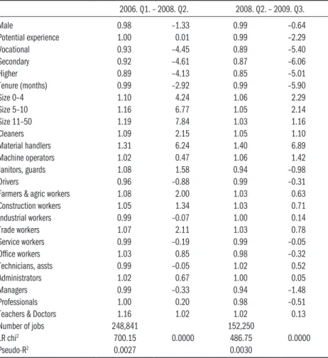
Following Jenkins (1995) we estimate discrete time duration models, in which members of two risk groups (employed and non-employed) are followed over time. The conditional job loss and job finding probabilities are estimated using constant and time-varying characteristics (X and Z) and time spent in the risk group (t) as explanatory variables. In equation (3) the term f(t) stands for a set of dummy variables denoting that the person was employed (non-em- ployed) for 1,2,…,T periods. In the case of employment t is measured in years of tenure in the current job as a continuous variable while in the case of non- employed individuals t is measured with dummies standing for the months of joblessness. The function g(τ) collects the parameters of a set of dummies measuring calendar time (quarters).

Pr (exit between t and t + 1 = βX + γZt + g(τ) + f(t) (3) Model (3) is estimated for a pool of 1.12 million observations from 2006.

Q1–2009.Q3. The 2010.Q1 wave of the LFS was not available at the writing of this text so we do not know the direction of exit from the populations ob- served in 2009.Q4. The observed period was split into two overlapping parts:

one from 2006.Q1 to 2008.Q2 and another from 2008.Q2 to 2009.Q3. Split- ting the period in this way has the advantage of observing if the parameters are the same before and during the crisis and ensuring that the calendar time ef- fects can be connected using 2008.Q2. as the reference wave in both periods.

The estimation results are presented in Appendix 2. Here we start with the calendar time effects shown in Figure 1.4. Surprisingly, we do not see a large in- crease in the rate of job loss during the crisis – flows out of employment jumped high in 2008 October – December but a similar hike could be observed one year earlier. The job loss rate followed an increasing trend throughout 2006–

2009, and the period of the crisis seems to fit the trend. By contrast, the job finding rate followed a decreasing trend in 2006–2008, and deteriorated mark- edly during the crisis.

Figure 1.4: The impact of calendar time on the probabilities of job loss and job finding (Logit odds ratios. Reference period: 2008.Q2.)

(a) Quarterly rates (b) Three-quarters moving average

Looking back in time, we observe a dramatic slump in the job finding rate in July-December 2006 that was most probably associated with the announc- ing of a strict austerity program in June and the outbreak of political unrest in September-October (panel a). It seems that in 2008, too, enterprises reacted to the arising uncertainties by drastically cutting hiring: in October-December the probability of escape from unemployment dropped to an exceptionally low level. Parts of the vacancies left open at the end of 2008 were most probably filled in January-March 2009, when the job finding rate jumped high tempo- rarily. If we smooth the zigzag by applying 3-quarters moving averages (panel b) the widening gap between the rates of job loss and job finding becomes eas- ily observable.

The slump in hiring strongly affected the baseline hazard of exit from non- employment (Figure 1.5). The baseline hazard captures how the risk of exit is affected by the duration of joblessness holding other observed characteristics constant.¹¹ The anti-clockwise shift of the baseline hazard curve at t=4 indi- cates that workers in the first four months of unemployment were less likely to get back to employment, and more likely to become long-term unemployed, in the period of the crisis.

The observed slump in hiring provides part of the explanation of why wage cuts and working time reductions did not play an important role in the adjust- ment to the crisis. Negotiations leading to soft measures are likely to develop if the jobs of many incumbents are at risk. The motivation for such negotia- tions is obviously weaker if firms react to the crisis by not replacing those, who retire or quit.

11 The hazard is also affected by unobserved attributes result- ing in a gradually growing share within an unemployed cohort of people with poor chance of exit.

Therefore the exit rate falls with the duration of joblessness even in the absence of “true” duration dependence.