PPCU Sam: Open-source face recognition framework

Procedia Computer Science 00 (2019) 000–000

www.elsevier.com/locate/procedia

23rd International Conference on Knowledge-Based and Intelligent Information & Engineering Systems

PPCU Sam: Open-source face recognition framework

Botos Csaba

, Hakkel Tamás

, András Horváth

, András Oláh

, István Z. Reguly

aPázmány Péter Catholic University Faculty of Information Technology and Bionics, Práter utca 50/a, Budapest 1083, Hungary

Abstract

In recent years by the popularization of AI, an increasing number of enterprises deployed machine learning algorithms in real life settings. This trend shed light on leaking spots of the Deep Learning bubble, namely the catastrophic decrease in quality when the distribution of the test data shifts from the training data. It is of utmost importance that we treat the promises of novel algorithms with caution and discourage reporting near perfect experimental results by fine-tuning on fixed test sets and finding metrics that hide weak points of the proposed methods. To support the wider acceptance of computer vision solutions we share our findings through a case-study in which we built a face-recognition system from scratch using consumer grade devices only, collected a database of 100k images from 150 subjects and carried out extensive validation of the most prominent approaches in single-frame face recognition literature. We show that the reported worst-case score, 74.3% true-positive ratio drops below 46.8% on real data.

To overcome this barrier, after careful error analysis of the single-frame baselines we propose a low complexity solution to cover the failure cases of the single-frame recognition methods which yields an increased stability in multi-frame recognition during test time. We validate the effectiveness of the proposal by an extensive survey among our users which evaluates to 89.5% true-positive ratio.

c

2019 The Author(s). Published by Elsevier B.V.

This is an open access article under the CC BY-NC-ND license (https://creativecommons.org/licenses/by-nc-nd/4.0/) Peer-review under responsibility of KES International.

Keywords: Face recognition; deep learning; real-world challenge; dataset generation; multi-frame verification; adaptation;

1. Introduction

Neural Networks. Artificial Neural Networks, been around for several decades as an alternative to classic Machine Learning algorithms, originally motivated by dynamic models of the biological brain. It was well-recognized for its ability to extract relevant patterns without manual tuning of the weights and biases of the network; however, the idea of the perceptron model has been frozen because it is proven to be unable to learn some elementary logic operations (like the XOR operation). The idea of neural networks has been frozen until the use of backpropagation (closely related to the Gauss-Newton algorithm) allowed the researchers to stack multiple perceptron layers (MLP) on the top of each

∗Corresponding authors. Tel.:+36-1-8864-717,+36-1-886-4764,+36-1-886-4764.

E-mail address:horvath.andras@itk.ppke.hu, olah.andras@itk.ppke.hu, reguly.istvan.zoltan@itk.ppke.hu 1877-0509 c2019 The Author(s). Published by Elsevier B.V.

This is an open access article under the CC BY-NC-ND license (https://creativecommons.org/licenses/by-nc-nd/4.0/) Peer-review under responsibility of KES International.

other. The problem with MLPs was the time complexity, since each forward pass between successive layers required a matrix multiplication.

The appearance of GPUs allowed the MLPs to be computed in parallel on multiple cores, which was mostly trivial to implement since the computation itself consists only elementary operations and involves no decision trees. In 2012 the ImageNet Large Scale Visual Recognition Competition [18] (ILSVRC) was won by a Convolutional Neural Network (CNN), called AlexNet [13], outperforming manually designed algorithms by a large margin. The success of AlexNet resulted in the current deep learning wave, that drew attention of professionals from different fields and connected them. The variety of the applications of deep neural networks (DNN) is wide, since they are universal approximators in theory, which means if enough training samples, computation time and capacity is provided, any function can be reconstructed and modeled. With the theory aside, the solution space of applied Neural Network has its own practical boundaries.

Data Collection. On the other hand, neural networks need huge amount of curated data, and building such a dataset can be as challenging as designing a network to process it. The main difficulty of collecting data is that one has to find a solution to make both recording and annotation fully automatic because the required size of dataset can be reached only that way. Lack of diversity within the dataset can be a problem, and also structuring, storing, maintaining, and searching data is not a trivial task. Additionally, the dataset to be learned by the algorithm is also changing in our case, as the system has to be able to learn faces of new users and even faces of registered users might slightly change.

To achieve this, our data collection system must be fast and robust, and the face recognition algorithm have to be adaptable.

Potentials. Besides the extensive work done on the field of computer vision and particularly face recognition, our case has some additional potentials that help our project to succeed. First, as we are not experts of access control systems, the existence of a working access control system at our University helped a lot to start our project. Also the number of people coming daily to our Faculty (∼300-400) is optimal, as it is high enough to provide a dataset that is sufficiently diverse and large, but not too high (in case much higher number of users it would be really difficult to store and maintain data and also much higher performance devices would be needed to record data). Finally, we were lucky to have such a supporting community of users who were open for new things and helped us by manually annotate their data.

2. Framework

Original Access Control System. When started developing the system, we took advantage of the existing access control system installed all over of our Faculty, and attached our hardware and software to it as an extension leaving the core system unmodified. That system is based on a simple and straightforward protocol: All students and employees have an card equipped with a passive RFID (Radio Frequency Identification) chip which holds a personal ID. That ID can be read by a card reader installed into the gate by the main entrance, and then that ID is transmitted to a remote access control server. That server checks the permission of the user, and sends enabling or denying signal back to the gate, opening or keeping locked the turnstiles.

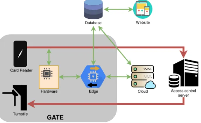
Our Extension. To accomplish our task we had to solve multiple task on multiple platforms. First, we have to collect raw data: record and save entries and camera pictures. Second, we need to register users and connect raw data with them. Third, we need to monitor incoming video stream to recognize faces of registered users. Finally, we need to make decisions (whether or not open the gate) and visualize output. Our system operates on 5 platforms, and figure1 displays these platforms and connectivity between them. The function of these platforms are the following:

• Microelectronics: Hardware that listens to the signals of the card reader and capable of emulating its signals, and also a microcontroller that connects hardware to Edge.

• Edge: A high performance embedded system located in the gate that serves as a relay center: 1) Receives data from Hardware and the web camera, 2) saves data from hardware to Database, 3) stream web camera photos to Cloud, 4) display photo stream coming back from Cloud, and 5) forward instructions coming from Cloud to Hardware.

Turnstile

Edge

GATE

Database Website

Access control server Card Reader

Cloud Hardware

Fig. 1: Overview of our extension, and connections between platforms.

• Cloud: A GPU server that processes images to find photos faces, match them to the ones already assigned to registered users, and make decision whether or not grant access permission.

• Website: A mobile friendly website that does the registration of new users, allow users to edit or delete their personal data, and provide an interface to annotate images (i.e. give feedback whether it shows the user which the photo is assigned to, or not).

• MySQL Database: Stores and retrieves temporary and persistent data, including photos, entry logs, user data, and annotations.

Our team has 4 developers: MITNYIK Levente and NASZLADY Márton Bese are responsible for the hardware part, BOTOS Csaba implemented programs running on Edge and Cloud, and HAKKEL Tamás designed and developed the Website and the Database. We have published the code base and hardware designs, and they are available here:

• Hardware design and respective source codes:https://dev.itk.ppke.hu/sam/gatepirate.git

• Edge and Cloud:https://github.com/botcs/sam

• Website:https://dev.itk.ppke.hu/sam/website.git

3. Dataset review

Public datasets. Many of the published face-recognition databases and corresponding benchmarks were inspired by the paper, Labeled Faces in the Wild (LFW) [7], which was released in 2007 with 5,749 subjects and 13,000 samples.

Since then, in parallel with the appearance of deep learning methods in big-data problems (such as the well-known Im- ageNET [3] challenges), the size of the face recognition databases has grown exponentially. The first open large-scale dataset, CelebFaces Attributes [14], commonly known as CelebA was published in 2014, featuring 10,177 celebrities on 202,599 photos. In late 2014, CASIA-WebFace dataset was published in the paper Learning face representation from scratch [21] with 494,414 images covering 10,575 identities. Next year, the original VGGFace dataset, de- scribed in the paper titled Deep Face Recognition [16] was released, listing 2,622 subjects on an exceptionally huge number of images, 2.6 million samples. The dataset had been revised and cleaned since its release and it contains 800,000 images with 305 samples per subject according to [1].

Quality over quantity. Exponential growth of the datasets has been receding since 2016, due to lagging growth of computation capacity. MegaFace [15] was released in 2016 with 4.7Mimages covering 672,057 subjects. Even though [15] contains high number of training samples, the image per identity ratio has an average of 7 face per person and reports>500kdistractor faces, which refers to an extremely challenging and mainly unrealistic setting. By the end of 2016, Microsoft published the MS-Celeb-1M (MS1M) dataset [4] that counts 10Mimages for 100ksubjects. Many papers studying various effects of altering the training conditions [17,20,8,2] report values on [4]. While MS- Celeb-1M is the largest publicly available dataset, its intra-class (or identity) variations is somewhat limited, due to the average 81 samples per subject and because of the relatively high error in the ground truth labels (samples were

collected using a search engine without manual correction). To study generalization capability of the algorithms two commonevaluation-onlydatasets, IARPA Janus Benchmark-A (IJB-A) [12] and Benchmark-B (IJB-B) [19] were released in 2015 and 2017 respectively. In 2018 VGGFace2 [1] (VF2) was released reporting a modest sized dataset with 3.3Mimages of 9,131 identities. Even though the size of the training set is limited, benchmarks of [1] show that face recognition networks trained on higher quality samples and labels with less noise outperforms those ones which were trained on [15,4], not just on the [1] validation set but the IJB-A [12] and IJB-B [19] benchmarks as well. In table1we summarize the statistics of the described datasets.

Sam Dataset overview. We started data collection by the middle of August of 2018. First, it was tested with a small number of users during summer break, but when the lectures started in September, our system was ready to handle multitude of new users. Unfortunately, from end of September until end of October, we had to suspend the operation of the system for technical reasons, so now there is 44 days (more exactly 332 hours) when we could record data. As of 25th of November, we have the following statistics:

• 171 registered user from both students and teachers.

• 98,224 photos of registered users, i. e.∼574 photo is belonging to a user on average. 82.4% of these images are identified by card swipe events, and 17.6% by the face recognition algorithm. On the most busy day, we captured 9,019 photos. Also, within a day there can be large differences in the number of recorded photos depending on the time of recording.

• 97.3% (95,601) of these photos are verified photos. Verification could be done either by card swipe event or manual annotation on the website. These verified images are used during face recognition as references.

Datasets # of subjects # of images # of images per subject manual year

LFW [7] 5,749 13,233 1/2.3/530 - 2007

CelebA [14] 10,177 202,599 -/19.9/- - 2014

CASIA-WebFace [21] 10,575 494,414 2/46.8/804 - 2014

IJB-A [12] 500 5,712 -/11.4/- - 2015

VGGFace [16] 2,622 2.6M 1,000/1,000/1,000 - 2015

MegaFace [15] 690,572 4.7M 3/7/2469 - 2016

MS-Celeb-1M [4] 100,000 10M -/100/- No 2016

IJB-B [19] 1,845 11,754 -/36.2/- - 2017

VGGFace2 [1] 9,131 3.3M 80/362.6/843 Partially 2018

PPCU-Sam (ours) 171 98,224 20/574/4048 Yes 2018

Table 1: Relevant entries are read from [1]. Empty values (denoted with dashes) were not reported by the authors. In the ’# of images per subject’

column min/avg/max values are represented respectively. Partial manual labeling refers to automated clustering where outliers were removed from the data. In contrast, our dataset consists of only manually approved labels, since each sample was accepted by its corresponding owner.

Partitioning the dataset. We divide the Sam dataset into four different categories:training,validation,test,underrep- resented. Firstly, we separate a high diversity set of identities that were covered by more than 50 images each, that sums up to 90ksamples. We shuffle the high diversity set and divide it up in 8 : 1 ratio fortraininingandvalidation purposes (we run a 9-fold cross validation, see the Implementation Details for further information). For thetestset we select identities, which represent well the scenario when a new user with short history is the subject of identification:

the number of samples from the person is>20 and≤50. We discard identities with images per subject≤20 since they areunderrepresentedand the reported benchmarks would have too high deviance.

4. Algorithm and evaluation methods

In our application the face recognition task is solved by a two step authentication: first we identify the user (one-to- many 1:N comparison), next we solve the verification task (one-to-one 1:1 comparison) using subsequent frames. In this chapter we describe the our core algorithm on the following levels: in Section4.1, we list recent works focusing on large scale face recognition and identification tasks, and report baseline evaluation of their performance on the

Sam dataset. In Section 4.2, we detail a robust, non-parametric multi-frame algorithm that treats the single-frame identification algorithm as a black-box predictor. Lastly, in Section4.3we describe the dynamically adapting search database that lets our users train the algorithm in real time.

4.1. Single-frame face identification

In this section we provide a detailed description of the identification problem, where a single, unknownqueryface is compared against agalleryof known faces, and how is this task is solved using embedding neural networks. The parameter optimization algorithms presented here form the core building blocks of most face-recognition systems and our main contribution in this work is a series of benchmarks with different performance metrics of the cutting edge training methods, implemented and evaluated on our dataset.

In our experiments we implement the state of the art algorithm that were used in evaluation of the VGGFace2 [1]

dataset. We use common performance metrics to report quantitative analysis on the difficulty of the Sam dataset comparable to others mentioned in3. We put a strong emphasis on our objective: we want to increase the performance of the best model on our dataset, to provide a reliable single-frame identification algorithm for our framework, and notto improve on the recent state of the art results on either external dataset.

Notation. Formally, in the space of images X ⊂ R^H×W×C we denote the learned distance metric ˆd : X × X → R between sample x1,x2 ∈ X, using an embedding function (our feature extractor) fθ: X → H, parametrized byθas the following: ˆd_θ(x₁,x₂)=d

f_θ(x₁),f_θ(x₂)

.In the equation abovedrepresents the distance metric that we are going to use in the learned E dimensional latent space H ⊂ R^E, formallyd : H × H → R. When we are identifying a querysamplex_qthan we compare it against a set of labeled samples (x_i,y_i), namely thegallery(x_i,y_i)∈ X × Yby the following steps: we evaluate each ˆd(xq,xi), then we create a candidate subset of identitiesC ⊆ Y, by defining it as "labels of those samples which are closer than threshold distance", formallyC={yi|yi∈ Y,d(xˆ q,xi)< }. Finally we count each identical labels’ occurrence inC, and define the predicted identity as the most frequent label among the candidate labels. For its simplicity and for comparable results with [1] we used Cross Entropy loss for training and cosine similarity for all of our experiments.

Architecture. Similarly to [1], for the backbone feature extractor we implemented the ResNet-50 (later referenced as ResNet) from Deep Residual Networks [5] and SE-ResNet-50 (later referenced as SENet) from Squeeze-and- Excitation Networks [6], winners of the Imagenet Large Scale Visual Recognition Challenge (ILSVRC) [18] 2015 and 2017 respectively. We measured performance under 3 setting for each architecture based on the dataset used for training:

(A) ResNet [5] trained on on MS1M [4] and finetuned on VF2 [1]

(B) SENet [6] trained on MS1M [4] and finetuned on VF2 [1]

(C) ResNet [5] from setting (A) finetuned on Sam (D) SENet [6] from setting (B) finetuned on Sam

(E) ResNet [5] trained on MS1M [4] and finetuned on Sam (F) SENet [6] trained on MS1M [4] and finetuned on Sam

Implementation details. For each cross-validation run we use 10ksamples from the high diversity set for validation and 80ksample for training, resulting ink=9-fold cross validation runs in total. By each run (except for setting A and B) we fine-tune the network in 20 epochs on thetrainingdata and save the state that performs best on thevalidation set, finally we use this state to evaluate scores ontest. All reported values on thetestset are computed as the arithmetic mean of the runs.

For each run, we evaluate TPIR and FPIR on thetestset using the following steps:

1. To get a list of similarity threshold values, we divide the (0,1] range using 5000 equally sized bins.

2. We compute the maximum number of hits by counting the labels in thegallerythat matches thequery.

3. To get the maxmimum number of misses, we take thegallerysize minus the the maximum number of hits.

4. We select samples that have higher similarity score than the given threshold value to obtain the list ofcandidates of the algorithm.

5. To obtain the total number of hits we measure how many of the candidate’s labels match thequery’s class.

6. To obtain the total number of misses we subtract the total number of hits from the size of the candidates.

7. To evaluate FPIR at a fixed threshold value we select the total number of hits and divide it with the maximum number of hits. To evaluate FPIR we do similarly.

For optimizing the embedding network we use Cross Entropy loss, Adam [11] optimizer with a fixed learning rate α= 0.005, with batch size of 128 on 224×224×3 images, cropped and aligned with dlib [10]. The output of the embedding network was 2048, for which we appliedL²normalization in test time. Similarly to [1], we used balancing strategy for each mini-batch due to the unbalanced nature of ourtraining data; Monochrome augmentation with probability of 0.2 to reduce over-fitting on colour images. We used pre-trained Caffe [9] weights from the authors [1], publicly available at:https://github.com/ox-vgg/vgg_face2. We trained and evaluated our models on 2×RTX- 2080 GPU.

4.2. Multi-frame face validation

In this section we introduce our model agnostic, non-parametric multi-frame face validation algorithm, that encap- sules the single-frame face identification algorithm, detailed in Section4.1. The goal is to validate whether the person identified first by the single-frame module can be assigned to a registered identity with high confidence.

Our aim with the presented design was to use the simplest possible approach to utilize the continuous stream of input. The basic idea is to treat the single-frame module as a probabilistic model, and draw multiple samples from the identification process and pass only if successful retrieval was repeated through multiple tests. We use the low temporal variance of the input samples to our advantage, improving the robustness of the final verification process, detailed in Algorithm:1. We note that the algorithm is vulnerable, for it relies heavily on the identification module’s success, however in practice this algorithm is the most straightforward to implement and its accuracy level satisfies our requirements.

Algorithm 1Sam Multi-frame verification. The algorithm returns and terminates only when the face is verified and the identity is not a distractor.

Require: f(x) .single frame identification function

Require: X .stream of frames

Require: N .# of successive retrieval

1: y←<UNK> .initialize identity value

2: counter←0 .initialize counter of successive retrievals

3: t←0 .initialize timestep

4: whilecounter<Ndo

5: t←t+1

6: x← X[t]

7: yˆ← f(x)

8: ifyˆ,<UNK>andyˆ=ythen

9: counter←counter+1

10: else

11: counter←0

12: y←yˆ returny

4.3. Dynamically adapting gallery

We enhance our system with the ability to extend the face database, or thegalleryon the fly by a user who wants to train the algorithm, and fine-tune the embedding networkf on the extended database later. To adapt to the changes in the search database we divide the tasks in to two categories. The first category is the on-line adaptation, detailed in Subsection4.3, while the second category is the off-line adaptation, detailed in Subsection4.3.

On-line adaptation. During on-line training, the main goal is to minimize the time between the identification and verification, by maximizing the precision and recall of the single-frame identifier.

In practice, the original samples of thegallery,xi are not stored on the device memory (by device we refer to the the GPU in thecloud), only their latent representationshi. During test time only the embedded code vector of thequeryimage is computed. This is detail is crucial from the aspect of real-time application, because its efficiency saves a tremendous amount of compute, and notable portion of the device memory, that leaves room for a dynamically growinggallery.

When users want to train the algorithm, they need to stand in the front of the camera and authenticate themselves using their unique ID badges. Then our application enters into the training state, which lasts until it loses track of the user using the face detection algorithm (a Convolutional Neural Network, implemented in dlib [10]). In the training state each inferred his automatically assigned to the identityy, added to thegallery. By doing so, the application increases the True Positive Identification Ratio of the identity, since the embeddings of successive frames have signif- icantly higher cosine similarity scores than negative and false positive samples. We note that we do not optimize the parametersθof the embedding function fθduring on-line training, and all the freshly added latent vectorshare stored locally on the device.

Using this approach, the time it takes to train the algorithm to identify and validate a new user on a decent level is reduced to 1 minute.

Off-line adaptation. When the face detection algorithm does not detect any face in the input stream for 2 seconds, we begin to synchronize the updatedgallerywith the SQL database, asynchronously with the face detector, which is allowed to interrupt the synchronization process any time. To increase sample diversity we only store every 3^rdimage of the user. After the synchronization process, the users can delete from the updated gallery on their personal site, also accept samples that wereverifiedby the algorithm. During weekends we fine-tune the embedding network on the latest available training samples in the SQL database. These manual changes take effect once every day (during night hours), by a completely separate process that loads the latest fine-tuned parameters of the network and compute the embedding vectors for every sample in the SQL database.

5. Results

5.1. Single-frame benchmarks

Performance metrics. We use different metrics to illustrate how the architecture and the different pre-training settings influence the outcome, namely:

• fixed False Positive Identification Ratio (FPIR)

• Rank-N vs. True Positive Identification Ratio (TPIR)

Results from the fixedFPIRbenchmark are shown in Table2a. In our case this is the most relevant metric, since it provides us information about the likelihood of identifying correctly thequerywith fixed likelihood of identifying an unknown person as a registered user. Results from theRank-Nbenchmark are listed in Table2b. To obtain Rank-N we measured the ratio of the retrieved true samples in the N Nearest Neighbour versus the total number of true samples in the gallery. For real time applications this metric is too expensive, because the ranking operation involves sorting the entiregalleryusing the similarity score that has a lower bound on the complexity in the worst case:nlognfor an nsizegallery. Also, because this metric is sensitive to the high variance of the image per identity ratio, it could be challenging to find an optimal threshold for identification. We used Nearest Neighbour search to make predictions for eachqueryimage. In general, the Top-k result refers to the case when the algorithm makeskguesses and we assume correct prediction if any of the guesses match the ground truth. We note that in our implementation each guess is allowed to belong to any of the identities.

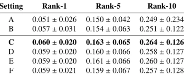
Observations. In Table2a and 2bwe notice that both the lowest and the highest scores were obtained by using ResNet [5]. The majority of the best results were achieved in setting C (described in Section4) in every benchmark, as the result of training the best performing model from [1], using MS1M and VGF and fine-tuning it on Sam-training.

The worst results were achieved by setting A, B, since they were not allowed to use any of the training samples, validating the usefulness of our limited training data.

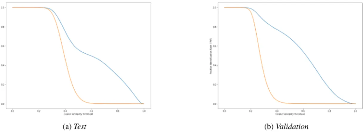
To illustrate the small differences ourtrainingdataset yields, we have plotted TPIR against FPIR on a logarithmic scale in the relevant FPIR range, (0,0.1] in Figure2a. In Figure2bwe compared the best performing setting (setting C) Receiver Operational Characteristic (ROC) curve on ourvalidationand on thetestset. In Figure3, plotting both the TPIR and the FPIR values against the cosine similarity threshold helps us determining the optimal threshold value for test time application. If we want to avoid false alarms (since it causes a serious security breach) we have to trade offretrieval of true matches, resulting in a less successful, or longer identification process. After careful consideration we set the cosine similarity threshold of the single-frame face detection algorithm to 0.6.

To emphasize the difficulty of the Sam-testset we compare the best results of the same algorithm (setting A) in Table3b. Notice the high variance of the same algorithm, and the difference in performance, it clearly shows the difficulty of the real world face-recognition task.

Setting FPIR=0.01 FPIR=0.05 FPIR=0.1 A 0.468±0.351 0.513±0.331 0.571±0.301 B 0.504±0.321 0.546±0.314 0.578±0.303 C 0.510±0.320 0.546±0.315 0.576±0.306 D 0.497±0.319 0.541±0.315 0.572±0.307 E 0.508±0.320 0.546±0.315 0.574±0.306 F 0.504±0.321 0.546±0.314 0.578±0.303

(a) True Positive Identification Ratios (TPIR) and correspond- ing standard deviance using fixed False Positive Identification Ratios (FPIR) on SAM-test set.

Setting Rank-1 Rank-5 Rank-10

A 0.051±0.026 0.150±0.042 0.249±0.234 B 0.057±0.031 0.154±0.063 0.251±0.122 C 0.060±0.020 0.163±0.065 0.264±0.126 D 0.059±0.020 0.160±0.066 0.258±0.127 E 0.059±0.020 0.161±0.066 0.260±0.127 F 0.059±0.021 0.159±0.067 0.257±0.128

(b) True Positive Identification Ratios using increasingkin the k-NN classification on the SAM-test set. We use cosine simi- larity for defining the inverse distance between the embedded features.

Table 2: Comparison of settings (A-E) using different metrics.

Dataset FPIR=0.01 FPIR=0.05 FPIR=0.1 Sam-training 0.736±0.316 0.789±0.300 0.812±0.286 Sam-validation 0.729±0.316 0.781±0.302 0.807±0.286 Sam-test 0.468±0.351 0.513±0.331 0.571±0.301

(a) Comparison of the best performing model (setting C) on thetrain,validationand thetestset. Notice that in real life sce- narios results are relevant for identities both in the validation and in the test set, since we the application is not restricted to trained and tested on different identities.

Dataset FPIR=0.01 FPIR=0.05 FPIR=0.1 IJB-B [19] 0.743±0.037 - 0.863±0.032 Sam-test(ours) 0.468±0.351 0.513±0.331 0.571±0.301

(b) Baseline evaluation of setting A on the IJB-B [19] dataset (read from [1], Table VII) and our testset. Notice the high variance of the same algorithm on our dataset compared to the low variation and the high scores on the IJB-B [19] evaluation dataset. This shows the difficulty of face recognition in real life applications.

Table 3: Difficulty comparisons.

5.2. User feedback on enhanced algorithm

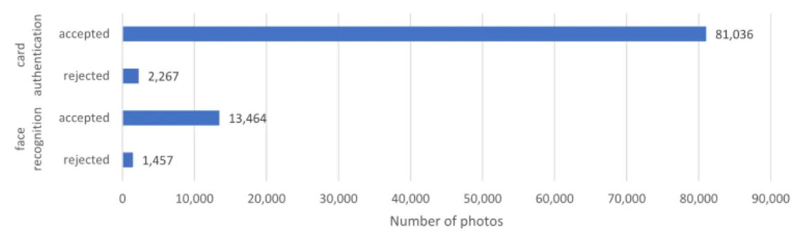
In contrast with the benchmarks made on single-frame identification, we were able to drastically increase perfor- mance using multi-frame validation and also by on-line and off-line adaptation. We validated the effectiveness of these proposals by an extensive survey among our users. Using the Website, we asked them to manually accept or reject the proposals of the recognition service, which accumulates to the following statistics:

• Card authentication (photos which were taken when the users entered the building using their card):

– 81,036 photos were accepted – 2,280 photos were rejected

• Face recognition:

– 14,617 photos were accepted – 1,717 photos were rejected

(a) TPIR vs. FPIR on a logarithmic scale. (b) ROC curve of setting C.

Fig. 2: Plotting the TPIR values against the FPIR scores yields the Receiver Operating Characteristic (ROC) curve. (left) Plotting different training settings reveals the small gains added by fine-tuning the network on the Sam-trainingset. (right) Depicting the difference between the validation and the test performance. The grey dashed line refers to the random guessing model. For the fixed FPIR comparison, see Table3a.

(a)Test (b)Validation

Fig. 3: TPIR (blue) and FPIR (orange) values plotted agains the Cosine similarity threshold results in a talkative characteristic: when the threshold

=0, every sample in thegalleryis accepted by the algorithm, therefore both TPIR and FPIR=1.0, while e.g. at threshold=0.6, the ratio of the retrieved negative samples (to the total number of negative samples) is respectably smaller than the ratio of the retrieved true samples (to the total number of true samples). Intuitively the aim is to increase the gap between TPIR and FPIR, by keeping false alarms as low as possible, or push the slope of the FPIR (orange) curve to the left as much as possible.

Fig.4visualizes the ratio of the groups these annotation outcomes. In conclusion, the ratio of accepted and rejected predictions of the face recognition algorithm is 89.48%, which we consider as the overall performance of the algo- rithm. The relatively high number of misclassified images in the "card authentication dataset" (i.e. the photos taken when the users entered the building using their card) lead us to the conclusion that there is some intrinsic source of error even in that methods that we attributed both to the mistakes of the photo-user matching algorithm and the non-regular behavior of the users (e.g. they used their card to let other people in).

6. Summary and discussion

Our goal was to build a real-life face-recognition application from scratch, using consumer grade devices and publicly available databases. In 44 days we collected 98,224 images that allowed us to perform a wide range of benchmarks using different metrics. To achieve the best performance we re-implemented state of the art single-frame recognition techniques and investigated failure cases of such approaches. In our experiments, we show that simply applying cutting edge methods on a custom dataset exposes the discrepancy between the reported worst-case perfor- mance 74.3%, and performance on the custom data 46.8%. By careful error analysis we designed a simple multi-frame identification process that substantially improves the effectiveness of the system, yielding a 89.5% true-positive per- formance ratio based on user feedback. The source

1,457

13,464 2,267

81,036

0 10,000 20,000 30,000 40,000 50,000 60,000 70,000 80,000 90,000

rejected accepted rejected accepted

face recognitioncard authentication

Number of photos

Fig. 4: User feedback. The first two rows display the number of annotations on images assigned to users by the algorithm that matches users and photos based on the timestamp of the photos and the time when users entered the building using their card. The last two rows show feedback on photos assigned to users by the face recognition algorithm ("unverified dataset"). Vast majority of these photos are confirmed by users that these images truly shows them.

References

[1] Qiong Cao et al. “Vggface2: A dataset for recognising faces across pose and age”. In:Automatic Face&Gesture Recognition (FG 2018), 2018 13th IEEE International Conference on. IEEE. 2018, pp. 67–74.

[2] Jen-Hao Rick Chang et al. “One Network to Solve Them All-Solving Linear Inverse Problems using Deep Projection Models.” In:ICCV.

2017, pp. 5889–5898.

[3] Jia Deng et al. “Imagenet: A large-scale hierarchical image database”. In:Computer Vision and Pattern Recognition, 2009. CVPR 2009.

IEEE Conference on. Ieee. 2009, pp. 248–255.

[4] Yandong Guo et al. “Ms-celeb-1m: A dataset and benchmark for large-scale face recognition”. In:European Conference on Computer Vision. Springer. 2016, pp. 87–102.

[5] Kaiming He et al. “Deep residual learning for image recognition”. In:Proceedings of the IEEE conference on computer vision and pattern recognition. 2016, pp. 770–778.

[6] Jie Hu, Li Shen, and Gang Sun. “Squeeze-and-excitation networks”. In:arXiv preprint arXiv:1709.015077 (2017).

[7] Gary B Huang et al. “Labeled faces in the wild: A database forstudying face recognition in unconstrained environments”. In:Workshop on faces in’Real-Life’Images: detection, alignment, and recognition. 2008.

[8] Rui Huang et al. “Beyond face rotation: Global and local perception gan for photorealistic and identity preserving frontal view synthesis”.

In:arXiv preprint arXiv:1704.04086(2017).

[9] Yangqing Jia et al. “Caffe: Convolutional architecture for fast feature embedding”. In:Proceedings of the 22nd ACM international conference on Multimedia. ACM. 2014, pp. 675–678.

[10] Davis E King. “Dlib-ml: A machine learning toolkit”. In:Journal of Machine Learning Research10.Jul (2009), pp. 1755–1758.

[11] Diederik P Kingma and Jimmy Ba. “Adam: A method for stochastic optimization”. In:arXiv preprint arXiv:1412.6980(2014).

[12] Brendan F Klare et al. “Pushing the frontiers of unconstrained face detection and recognition: Iarpa janus benchmark a”. In:Proceedings of the IEEE conference on computer vision and pattern recognition. 2015, pp. 1931–1939.

[13] Alex Krizhevsky, Ilya Sutskever, and Geoffrey E Hinton. “Imagenet classification with deep convolutional neural networks”. In:Advances in neural information processing systems. 2012, pp. 1097–1105.

[14] Ziwei Liu et al. “Deep Learning Face Attributes in the Wild”. In:Proceedings of International Conference on Computer Vision (ICCV).

Dec. 2015.

[15] Daniel Miller et al. “Megaface: A million faces for recognition at scale”. In:arXiv preprint arXiv:1505.02108(2015).

[16] O. M. Parkhi, A. Vedaldi, and A. Zisserman. “Deep Face Recognition”. In:British Machine Vision Conference. 2015.

[17] Rajeev Ranjan, Carlos D Castillo, and Rama Chellappa. “L2-constrained softmax loss for discriminative face verification”. In:arXiv preprint arXiv:1703.09507(2017).

[18] Olga Russakovsky et al. “Imagenet large scale visual recognition challenge”. In:International Journal of Computer Vision115.3 (2015), pp. 211–252.

[19] Cameron Whitelam et al. “IARPA Janus Benchmark-B Face Dataset.” In:CVPR Workshops. Vol. 2. 5. 2017, p. 6.

[20] Xiang Wu et al. “A light CNN for deep face representation with noisy labels”. In:IEEE Transactions on Information Forensics and Security 13.11 (2018), pp. 2884–2896.

[21] Dong Yi et al. “Learning face representation from scratch”. In:arXiv preprint arXiv:1411.7923(2014).