for Kernel Methods by Gradient Perturbations
Bal´azs Csan´ad Cs´aji · Kriszti´an Bal´azs Kis
Abstract We propose a data-driven approach to quantify the uncertainty of mod- els constructed by kernel methods. Our approach minimizes the needed distribu- tional assumptions, hence, instead of working with, for example, Gaussian pro- cesses or exponential families, it only requires knowledge about some mild regu- larity of the measurement noise, such as it is being symmetric or exchangeable. We show, by building on recent results from finite-sample system identification, that by perturbing the residuals in the gradient of the objective function, information can be extracted about the amount of uncertainty our model has. Particularly, we provide an algorithm to build exact, non-asymptotically guaranteed, distribution- free confidence regions for ideal, noise-free representations of the function we try to estimate. For the typical convex quadratic problems and symmetric noises, the regions are star convex centered around a given nominal estimate, and have effi- cient ellipsoidal outer approximations. Finally, we illustrate the ideas on typical kernel methods, such as LS-SVC, KRR,ε-SVR and kernelized LASSO.
Keywords kernel methods · confidence regions · nonparametric regression · classification·support vector machines·distribution-free methods
Bal´azs Csan´ad Cs´aj EPIC Centre of Excellence
MTA SZTAKI: Institute for Computer Science and Control Hungarian Academy of Sciences, Budapest, Hungary Tel.: +(36)-1-279-6231 Fax: +(36)-1-279-7503 E-mail: balazs.csaji@sztaki.mta.hu
Kriszti´an Bal´azs Kis EPIC Centre of Excellence
MTA SZTAKI: Institute for Computer Science and Control Hungarian Academy of Sciences, Budapest, Hungary Tel.: +(36)-1-279-6111 Fax: +(36)-1-279-7503 E-mail: krisztian.kis@sztaki.mta.hu
1 Introduction
Kernel methods build on the fundamental concept of Reproducing Kernel Hilbert Spaces (Aronszajn, 1950; Gin´e and Nickl, 2015) and are widely used in machine learning (Shawe-Taylor and Cristianini, 2004;Hofmann et al.,2008) and related fields, such as system identification (Pillonetto et al.,2014). One of the reasons of their popularity is the representer theorem (Kimeldorf and Wahba,1971;Sch¨olkopf et al.,2001) which shows that finding an estimate in an infinite dimensional space of functions can be traced back to a finite dimensional problem. Support vector machines (Sch¨olkopf and Smola,2001;Steinwart and Christmann,2008), rooted in statistical learning theory (Vapnik,1998), are typical examples of kernel methods.
Besides how to construct efficient models from data, it is also a fundamental question how to quantify theuncertaintyof the obtained models. While standard approaches like Gaussian processes (Rasmussen and Williams,2006) or exponential families (Hofmann et al.,2008) offer a nice theoretical framework, making strong statistical assumptions on the system is sometimes unrealistic, since in practice we typically have very limited knowledge about the noise affecting the measurements.
Building on asymptotic results, such as limiting distributions, is also widespread (Gin´e and Nickl,2015), but they usually lack finite sample guarantees.
Here, we propose a non-asymptotic,distribution-freeapproach to quantify the uncertainty of kernel-based models, which can be used forhypothesis testing and confidence regionconstructions. We build on recent developments in finite-sample system identification (Campi and Weyer,2005;Car`e et al.,2018), more specifically, we build on the Sign-Perturbed Sums (SPS) algorithm (Cs´aji et al.,2015) and its generalizations, the Data Peturbation (DP) methods (Kolumb´an,2016).
We consider the case where there is an underlying “true” function that gener- ates the measurements, but we only have noisy observations of its outputs. Since we want to minimize the needed assumptions, for example, we do not want to assume that the true underlying function belongs to the Hilbert space in which we search our estimate, we take a “honest” approach (Li,1989) and consider “ideal”
representations of the target function from our function space. A representation is ideal w.r.t. the data sample, if its outputs coincide with the corresponding (hidden) noise-free outputs of the true underlying function for all available inputs.
Despite our method isdistribution-free, i.e., it does not depend on any param- eterized distributions, it has strong finite-sample guarantees. We argue that, the constructed confidence region contains the ideal representationexactlywith a user- chosen probability. In case the noises are independent and symmetric about zero, and the objective function is convex quadratic, the resulting regions arestar con- vexand have efficientellipsoidal outer approximations, which can be computed by solving semi-definite optimization problems. Finally, we demonstrate our approach on typical kernel methods, such as KRR, SVMs and kernelized LASSO.
Our approach has some similarities to bootstrap (Efron and Tibshirani,1994) and conformal prediction (Vovk et al.,2005). One of the fundamental differences w.r.t bootstrap is, e.g., that we avoid building alternative samples and fitting bootstrap estimates to them (since it is computationally challenging), but perturb directly the gradient of the objective function. Key differences w.r.t. conformal prediction are, e.g., that we want to quantify the uncertainty of the model and not necessarily that of the next observation (though the two problems are related), and more importantly, exchangeability is not fundamental for our approach.
2 Preliminaries
A Hilbert space,H, of functionsf :X →R, with inner producth·,·iH, is called a Reproducing Kernel Hilbert Space(RKHS), if the point evaluation functional
δz:f→f(z), (1)
is continuous (or equivalently bounded) for all z ∈ X, at any f ∈ H(Gin´e and Nickl,2015). Then, by using the Riesz representation theorem, one can construct a (unique) kernel,k:X × X →R, having thereproducingproperty, that is
hk(·, z), fiH = f(z), (2) for allz∈ X andf∈ H. In particular, the kernel satisfies for allz, s∈ X that
k(z, s) = hk(·, z), k(·, s)iH. (3)
Hence, the kernel of an RKHS is a symmetric and positive-definite function; more- over, the Moore-Aronszajn theorem states that the converse is also true: for every symmetric, positive-definite function there is a unique RKHS (Aronszajn,1950).
Typical kernels include, e.g., the Gaussian kernel k(z, s) = exp(−kz−sk2/2σ2), with σ >0, the polynomial kernel,k(z, s) = (hz, si+c)p, withc≥0 and p∈N, and the sigmoidal kernel,k(z, s) = tanh(ahz, si+b) for somea, b≥0, where h·,·i denotes the standard Euclidean inner product (Hofmann et al.,2008).
By adata sample,Dn, we mean a finite set of input-output measurements, (x1, y1), . . . , (xn, yn) ∈ X ×R, (4) with X 6=∅. We also introducex .
= (x1, . . . , xn)T∈ Xn andy .
= (y1, . . . , yn)T∈ Rn. TheGram matrixofk(·,·), w.r.t. inputx, is denoted by Kx∈Rn×n, where
[ Kx]i,j .
= k(xi, xj). (5)
A kernel is called strictly positive definite if its Gram matrix, Kx, is (strictly) positive definite fordistinctinputs{xi} (Hofmann et al.,2008).
One of the fundamental reasons for the successes of kernel methods is the so- called representer theorem, originally given byKimeldorf and Wahba(1971), but the generalization presented here is due toSch¨olkopf et al.(2001).
Theorem 1 Suppose we are given a sample,Dn, a positive-definite kernelk(·,·), an associated RKHS with a normk · kHinduced byh·,·iH, and a class of functions
F .
= n
f :X →R | f(z) =
∞
X
i=1
βik(z, zi), βi∈R, zi∈ X,kfkH<∞o , (6) then, for any monotonically increasing regularization function,Λ : [0,∞)→[0,∞), and an arbitrary loss functionL : (X ×R2)n→R∪ {∞}, the objective
g(f,Dn) .
= L (x1, y1, f(x1)), . . . ,(xn, yn, f(xn))
+ Λ(kfkH), (7) has a minimizer admitting the following representation
fα(z) =
n
X
i=1
αik(z, xi), (8)
whereα .
= (α1, . . . , αn)T∈Rn is the vector of coefficients. IfΛ is strictly mono- tonically increasing, then each minimizer admits a representation having form(8).
The theorem can be extended with a bias term (Sch¨olkopf and Smola, 2001), in which case if the solution exists, it also contains a multiple of the bias term.
For further generalizations, see (Yu et al.,2013;Argyriou and Dinuzzo,2014).
The power of the representer theorem comes from the fact that it shows that computing the point estimate in a high, typically infinite, dimensional space of models can be reduced to a much simpler (finite dimensional) optimization problem whose dimension does not exceed the size of the data sample we have, that isn.
If the data is noisy, then of course, the obtained estimate is arandomfunction and it is of natural interest to study thedistributionof the resulting function, for example, to evaluate itsuncertaintyor to testhypothesesabout the system.
3 Confidence Regions for Kernel Methods
Now, we turn our attention to a stochastic variant of the problem discussed above.
There are several advantages of taking a statistical point of view on kernel meth- ods, including conditional modeling, dealing with structured responses, handling missing measurements and building prediction regions (Hofmann et al.,2008).
Following a standard statistical viewpoint (Davies et al.,2009), we assume that the outputs{yi}are generated by some noisy observations of an underlying “true”
function, denoted byf∗, that is for alli= 1, . . . , n, the outputs can be written as yi .
= f∗(xi) +εi, (9)
where{εi}are the noise terms. The entire noise vector isε .
= (ε1, . . . , εn)T. The noiseless outputs of functionf∗ will be denote byy∗i .
=f∗(xi), fori= 1, . . . , n.
3.1 Ideal Representations
We aim atquantifying the uncertaintyof our estimated model. A standard way to measure the quality of a point-estimate is to build confidence regionsaround it.
However, it is not obvious what we should aim for with our confidence regions.
For example, since all of our models live in our RKHS,H, we would like to treat the confidence region as a subset of H. On the other hand, we want to minimize the assumptions, for example, we may not want to assume thatf∗ is an element ofH. Furthermore, since unless we make strong smoothness assumptions on the underlying unobserved function, we only have information about it at the actual inputs,{xi}. Hence, we aim for a “honest” nonparametric approach (Li,1989) and search for functions which correctly describe the hidden function,f∗, on the given inputs. Then, by the representer theorem, we may restrict ourselves to a finite dimensional subspace ofH. This leads us to the definition ofideal representations:
Definition 1 Let Hα ⊆ H denote the subspace of functions that can be repre- sented as (8). A functionf0∈ Hα, having coefficientsα0∈Rn, is called an ideal or noise-free representation of the “true” unobserved functionf∗, if we have
f0(xi) = yi∗ .
= f∗(xi), for all i∈ {1, . . . , n}. (10) The set of all ideal representations, w.r.t. data sampleDn, is denoted byH0⊆ Hα, and the set of their coefficients, calledideal coefficients, is denoted byA0⊆Rn.
An ideal representation does not simply interpolate the observed (noisy) out- puts{yi}, but it interpolates theunobserved(noise-free) outputs, that is{y∗i}.
A natural question which arises is: when does such an ideal representation exist? To answer this question, first note that since ideal representations have the form (8), equation system (10) can be rewritten in a matrix form by using the Gram matrix. That is, vectorαis an ideal coefficient vector, if and only if
Kxα = y∗, (11)
wherey∗ .
= (y1∗, . . . , yn∗)T. If Kxis (strictly) positive definite, which is the case if for example the kernel is Gaussian and all inputs are distinct, then rank(Kx) =n andevery f∗:X →Rhas auniqueideal representation w.r.t. data sampleDn.
On the other hand, if rank(Kx) < n, then (11) places a restriction on the functions which have ideal representations. For example, ifX =Rand ker(z, s) = hz, si = zTs, then rank(Kx) = 1 and in general only functions which are linear on the data sample have ideal representations. This is of course not surprising, as it is well-known that the choice of the kernel encodes our inductive bias on the underlying true function we aim at estimating (Sch¨olkopf and Smola,2001).
If rank(Kx)< nand there is anαwhich satisfies (11), then there are infinitely many ideal representations, as for allν∈null(Kx), the null space of Kx, we have Kx(α+ν) = Kxα+ Kxν = Kxα = y∗.The opposite is also true, ifαandβboth satisfy (11), then Kx(α−β) = Kxα− Kxβ = 0, thus,α−β∈null(Kx). Hence, to avoid allowing infinitely many ideal representations, we may formequivalence classes by treating coefficient vectorsα andβ equivalent if Kxα = Kxβ. Then, we can work with the resultingquotient spaceof coefficients to ensure that there is only one ideal representation (i.e., one equivalence class of such representations).
All of our theory goes trough if we work with the quotient space of represen- tations, but to simplify the presentation we make the assumption (cf. Section4.2) that Kxis full rank, therefore, there alwaysuniquely existsan ideal representation (for any “true” function), whose unique coefficient vector will be denoted byα∗. 3.2 Exact and Honest Confidence Regions
Let (Ω,A,{Pθ}θ∈Θ) be astatistical space, where Θ denotes an arbitraryindex set.
In other words, for all θ ∈ Θ, (Ω,A,Pθ) is a probability space, where Ω is the sample space,Ais theσ-algebra of events, andPθ is a probability measure. Note that it isnot assumedthat Θ⊆Rd, for somed; therefore, this formulation covers nonparametricinference, as well (and that is why we do not callθa “parameter”).
In our case, indexθ is identified with the underlying true function, therefore, each possible f∗ induces a different probability distribution according to which the observations are generated. Confidence regions constitute a classical form of statistical inference, when we aim at constructing sets which cover with high prob- ability some target function of θ (DeGroot and Schervish, 2012). These sets are usually random as they are typically built using observations. In our case, we will build confidence regions for the ideal coefficient vector (equivalently, the ideal representation), which itself is a random element, as it depends on the sample.
Let γ be a random element (it corresponds to the available observations), let g(θ, γ) be some target function of θ (which can possibly also depend on the observations) and let p ∈ [ 0,1 ] be a target probability, also called significance
level. A confidence region forg(θ, γ) is a random set,C(p, γ)⊆range(g), i.e., the codomain of function g. The following definition formalizes two important types of stochastic guarantees for confidence regions (Davies et al.,2009).
Definition 2 A confidence regionC(p, γ) forg(θ, γ) is calledexact, if
∀θ∈Θ :Pθ(g(θ, γ)∈C(p, γ) ) = p, (12) and it is calledhonest, if it satisfies ∀θ∈Θ :Pθ(g(θ, γ)∈C(p, γ) ) ≥ p.
In our case,γis basically1the sample of input-output pairs,Dn; and the target object we aim at covering isg(θ, γ) =α∗θ, i.e., the (unique) ideal coefficient vector corresponding to the underlying true function (identified by θ) and the sample.
Since the ideal coefficient vector uniquely determines the ideal representation (to- gether with the inputs, which however we observe), it is enough to estimate the former. The main question of this paper is how can we construct exact or honest confidence regions for the ideal coefficient vector based on a finite sample without strong distributional assumptions on the statistical space.
Henceforth, we will treatθ(the underlying true function) fixed, and omit theθ indexes from the notations, to simplify the formulas. Therefore, instead of writing Pθorα∗θ, we will simply usePorα∗. The results are of course valid for allθ.
Standard ways to construct confidence regions for kernel-based estimates typ- ically either makestrong distributional assumptions, like assuming Gaussian pro- cesses (Rasmussen and Williams, 2006), or resort to asymptotic results, such as Donsker-type theorems for Kolmogorov-Smirnov confidence bands. An alterna- tive approach is to build on Rademacher complexities, which can provide non- asymptotic, distribution-free confidence bands (Gin´e and Nickl,2015). Neverthe- less, these regions are conservative (not exact) and are constructed independently of the applied kernel method. In contrast, our approach provides exact, non- asymptotic,distribution-freeconfidence sets for auser-chosenkernel estimate.
4 Non-Asymptotic, Distribution-Free Framework
This section presents the proposed framework to quantify the uncertainty of kernel- based estimates. It is inspired by and builds on recent results from finite-sample system identification, such as the SPS and DP methods (Campi and Weyer,2005;
Cs´aji et al.,2015;Cs´aji,2016;Kolumb´an,2016;Car`e et al.,2018). Novelties with respect to these approaches are, e.g., that our framework considersnonparametric regression and does not require the “true” function to be in the model class.
4.1 Distributional Invariance
The proposed method is distribution-free in the sense that it does not presup- pose any parametric distribution about the noise vectorε. We only assume some mild regularity about the measurement noises, more precisely that their (joint) distribution is invariant with respect to a known group of transformations.
1 We used the word “basically”, since there will also be some other random elements in the construction, e.g., for tie-breaking, and those should also constitute part of observationγ.
Definition 3 An Rn-valued random vector v is distributionally invariant with respect to a compactgroup of transformations, (G,◦), where “◦” is the function composition and each G ∈ G maps Rn to itself, if for all transformationG ∈ G, random vectorsv andG(v) have the same distribution.
The two most important examples of the above definition are as follows.
– If{εi} areexchangeable random variables, then the (joint) distribution of the noise vectorεis invariant w.r.t. multiplications by permutation matrices (which are orthogonal and form a finite, thus compact, group).
– On the other hand, if{εi}are independent, each having a (possibly different!) symmetricdistribution about zero, then the (joint) distribution ofεis invari- ant w.r.t. multiplications by diagonal matrices having +1 or −1 as diagonal elements (which are also orthogonal, and form a finite group).
Both of these examples assume only mild regularities about the measurement noises: for example, it is a standard assumption in statistical learning theory that the sample is independent and identically distributed (i.i.d.) which immediately implies exchangeability (which is a more general concept than i.i.d.). But even this assumption can be omitted if we work with symmetric noises, which are widespread as most standard distributions in statistics are symmetric, such as Gauss, Laplace, Cauchy, Student’s t, uniform, plus a large class of multimodal ones.
Note that for these examples no assumptions about other properties of the (noise) distributions are needed, e.g., they can beheavy-tailed, with eveninfinite variance, skewed, their expectations need not exist, hence,no moment assumptions are necessary. For the case of symmetric distributions, it is even allowed that the observations are affected by a noise where eachεi has a differentdistribution.
4.2 Main Assumptions
Before the general construction of our method is explained, first, we highlight the core assumptions we apply. We also discuss their relevance and implications.
Assumption 1 The kernel,k(·,·), is strictly positive definite and all inputs,{xi}, are distinct with probability one(in other words, ∀i6=j:P(xi=xj) = 0 ).
As we discussed in Section3.1, this assumption ensures that rank(Kx) =n(a.s.), hence thereuniquely exists an ideal representation (a.s.), whose unique ideal co- efficient vector is denoted by α∗. The primary choices are universal kernels for whichHis dense in the space of continuous functions on compact domains ofX. Assumption 2 The input vectorxand the noise vector εare independent.
Assumption 2 implies that the measurement noises, {εi}, do not affect the inputs,{xi}; for example, the system is not autoregressive. It is possible to extend our approach to dynamical systems, e.g., using similar ideas as in (Cs´aji et al., 2012; Cs´aji and Weyer, 2015; Cs´aji,2016), but we leave the extension for future research. Note that Assumption2allows deterministic inputs, as a special case.
Assumption 3 Noiseεis distributionally invariant w.r.t. a known group of trans- formations,(G,◦), where eachG∈ G acts onRnand◦is the function composition.
Assumption 3 states that we known transformations that do not change the (joint) distribution of the measurement noises. As it was discussed in Section4.1, symmetry and exchangeablity are two standard examples for which we know such group of transformations. Thus, if the noise vector is either exchangeable (e.g., it is i.i.d.), or symmetric, or both properties hold, then the theory applies. We also note that the suggested methodology is not limited to exchangeabe or symmetric noises, e.g., power defined noises constitute another example (Kolumb´an,2016).
Assumption 4 The gradient, or a subgradient, of the objective w.r.t.αexists and it only depends on the output vector, y, through the residuals, i.e., there is ¯g,
∇αg(fα,Dn) = ¯g(x, α,ε(x, y, α)),b (13) where the residuals w.r.t. the sample and the coefficients are defined as
ε(x, y, α)b .
= y − Kxα. (14)
For Assumption4, it is enough if a subgradient is defined for each coefficient vector α, hence, e.g., the cases of ε-insensitiveandHuber loss functions are also covered. Even in such cases (when we work with subderivaties), we still treat ¯gas a vector-valued function and choose arbitrarily from the set of possible subgradients.
This requirement is also very mild as it is typically the case that the objective function is differentiable or convex and has subgradients (we will present several demonstrative examples in Section 5); furthermore, the objective typically only depends onythrough the residuals, which immediately imply Assumption4.
To see this assume thatgis differentiable; then clearly, if the objective function can be written asg(fα,Dn) = g0(x, α,bε(x, y, α)) for some functiong0, then
∇αg(fα,Dn) = ∇α(g0(x, α, y−Kxα)))
= −Kx(∇αg0) (x, α, y−Kxα))
= ¯g(x, α,ε(x, y, α)),b (15)
where during the derivation we applied the chain rule, used the fact that matrix Kx is symmetric and the definition of the residuals,ε(x, y, α) =b y−Kxα.
4.3 Perturbed Gradients
At first, the proposed method can be understood as ahypothesis testingapproach.
Given coefficient vectorα∈Rnwe test the null hypothesisH0:α = α∗, i.e., it is the ideal coefficient vector; against the alternative hypothesisH1:α 6= α∗. Under H0, the residuals of fα coincide with the “true” (unobserved) noise terms, since by definition (for ideal representations), we have
bε(x, y, α∗) = y − Kxα∗
= [f∗(x1) +ε1, . . . , f∗(xn) +εn]T
− [f∗(x1), . . . , f∗(xn) ]T = ε. (16) Consequently, based on the group of invariant transformations,G, we know that the (joint) distribution of the residuals does not change if we transform them by
anyG∈ G (underH0). Then, we can generate alternative realizations of the resid- uals, ε(x, y, αb ∗), by applying a random transformationG ∈ G, and the resulting alternative realization, G(ε(x, y, αb ∗)), will behave “similarly” (in the statistical sense) to the original residual vector (i.e., the true noise vector).
However, under H1, if coefficient vector α does not define an ideal represen- tation,ε(x, y, α), in general, will not coincide with the true noises. Therefore, theb distributions of their randomly transformed variants will be distorted and will statisticallynot behave “similarly” to the original residuals.
Of course, we need a way to measure “similar behavior”. Since we want to measure the uncertainty of a model constructed by using a certain objective func- tion, we will measure similarity by recalculating (the magnitude of) its gradient (w.r.t.α) with the transformed residuals and apply a rank test (Good,2005).
Let us define areferencefunction,Z0:Rn→R, andm−1perturbedfunctions, {Zi}, withZi:Rn→R, wheremis a user-chosen hyper-parameter, as follows
Z0(α) .
= kΨ(x) ¯g(x, α, G0(ε(x, y, α)))b k2, (17) Zi(α) .
= kΨ(x) ¯g(x, α, Gi(bε(x, y, α)))k2, (18) for i = 1, . . . , m−1, where Ψ(x) is some (possibly input dependent) positive definite weighting matrix, G0 is the identity element of G (w.l.o.g. the identity transformation), and{Gi}are i.i.d. random transformations fromG, sampled using the uniform distribution on G. They are generated independently of the other random elements of the system, such as the input vectorxand the noise vectorε.
For symmetric noises, transformation Gi ∈ G is basically a random n×n diagonal matrix whose diagonal elements are +1 or−1, each having1/2probability to be selected, independently of the other elements of the diagonal.
On the other hand, for the case of exchangeable noise terms, each transforma- tionGi ∈ G is a randomly (uniformly) chosenn×npermutation matrix.
Weighting matrix Ψ(x) is included in the construction to allow some additional flexibility, e.g., if we have some a priori information on the measurement noises.
We will see an example for the special case of quadratic objectives in Section4.6.
In case no such information is available, Ψ(x) can be chosen as identity.
We can observe that for the ideal coefficient vectorα∗, we have Z0(α∗) = kΨ(x) ¯g(x, α∗, ε)k2
=d kΨ(x) ¯g(x, α∗, Gi(ε))k2
= Zi(α∗), (19)
for i = 1, . . . , m−1, where ,,=” denotes equality in distribution. Therefore, thed {Zi(α∗)}m−1i=0 variables have the same (marginal) distribution, though, they are of course not independent. It can be shown, however, that they areconditionally independent, and therefore all of their possible orderings are equally likely, with possible tie-breakings, which can be used to measuresimilarbehavior.
On the other hand, forα6=α∗, this distributional equivalence does not hold, and we expect that if kα−α∗kis large enough, the reference elementZ0(α) will dominate the perturbed elements,{Zi(α)}m−1i=1 , with high probability, from which we can detect (statistically) that coefficient vectorαis not the ideal one,α6=α∗.
4.4 Normalized Ranks
Now, we make our argument, including possible tie-breakings, more precise by introducing the concept of normalized ranks. Formally, thenormalized rankof the reference element,Z0(α), among all{Zi(α)}m−1i=0 elements is defined as follows
R(α) .
= Rm(α) .
= 1 m
1 +
m−1
X
i=1
I(Z0(α)≺πZi(α))
, (20)
whereI(·) is an indicator function, namely, its value is 1 if its argument is true and 0 otherwise;m∈Nis a user-chosen hyper-parameter; and binary relation “≺π” is the standard “<” with random tie-breaking (according to a fixed, pre-generated random order). More precisely, letπbe a random (uniformly chosen) permutation of the set{0, . . . , m−1}. Then, given m arbitrary real numbers,Z0, . . . , Zm−1, we can construct a strict total order, denoted by “≺π”, by definingZk ≺π Zj if and only ifZk< Zj or it both holds thatZk=Zj andπ(k)< π(j).
4.5 Exact Confidence
Parameterminfluences the resolution of the confidence probability we can achieve.
Namely, a probability p∈ (0,1) is admissible if it can be written in the form of p= 1−q/m, whereqis an integer satisfying 0< q < m. On the other hand, since bothmandqare (hyper) parameters, their values are user-chosen. Hence, every rational probability p ∈(0,1) is admissible, by choosing m andq appropriately.
Then, a confidence set for an admissible probabilityp=p(m, q) is Ap .
= {α:R(α)≤p} = {α:Rm(α)≤1−q/m}. (21) One of the main questions is: what kind of stochastic guarantees do such con- fidence regions have? The following theorem states that they areexact.
Theorem 2 Under Assumptions 1, 2, 3 and 4, the coverage probability of the constructed confidence region with respect to the ideal coefficient vectorα∗ is
P α∗∈Ap
= p = 1− q
m, (22)
for any choice of the integer hyper-parameters satisfying 0 < q < m.
Proof Following (Cs´aji et al.,2015), the core idea is to show that variables Z0(α∗), Z1(α∗), . . . , Zm−1(α∗) (23) are uniformly ordered, which means that each ordering of them, with respect to the strict total order≺π, has the same probability, that is 1/m!, formally,
P Zi0(α∗)≺πZi2(α∗)≺π · · · ≺πZim−1(α∗)
= 1
m!, (24)
where (i0, i1, . . . , im−1) is an arbitrary permutation of (0,1, . . . , m−1). This or- dering property is not obvious, since they are not independent, even though we already observed that they are identically distributed (for ideal coefficients).
By definition,α∗∈Ap if and only ifR(α∗)≤1−q/m, i.e., if the reference ele- ment,Z0(α∗) takes one of the positions 1, . . . , m−qin the ordering of{Zi(α∗)}m−1i=0 variables, w.r.t. the strict total order≺π. Then, assuming they are uniformly or- dered (yet to be shown), we know thatZ0(α∗) takes each position in the ordering with probability exactly 1/m. Therefore, fori∈ {1, . . . , m}, we have
P
R(α∗) = i m
= 1
m, (25)
from which it follows that P α∗ ∈ Ap
= 1−q/m by taking into account that events{ R(α∗) =i/m}and{ R(α∗) =j/m}are disjoint, ifi6=j.
In order to show that{Zi(α∗)}m−1i=0 are indeed uniformly ordered, we can apply Theorem 2.17 of (Kolumb´an,2016). Our proposed approach can be interpreted as a variant of a DP method, even though formally the DP “performance measures”
can depend on the parameters,α, the inputs,x, and the perturbed outputs,y(i), but not directly on the perturbed residuals. Nevertheless, in our case,y(i)is
y(i) .
= fα(x) + Gi(bε(x, y, α)), (26) wherefα(x) .
= [fα(x1), . . . , fα(xn)]T. Then, obviously we can compute the trans- formed residuals,Gi(ε(x, y, α)), fromb α,x, andy(i)by using thatGi(ε(x, y, α)) =b y(i)−fα(x). Hence, the DP performance measure in our case is defined as
Z(α, x, y(i)) .
= kΨ(x) ¯g(x, α, y(i)−fα(x))k2, (27) which now fits the DP framework. Our Assumption4ensures that this function is well-defined and, together with Assumption2, it also guarantees that we do not need to compute {y(i)} to evaluate the perturbed functions. Our Assumption 3 directly states that the noise,ε, is invariant under a compact group of transforma- tions, which is a requirement of Theorem 2.17, and we already observed that true errors coincide with the residuals of ideal representations,bε(x, y, α∗) = ε. ut Theorem2shows that the confidence region contains the ideal coefficient vector exactlywith probabilitypthat statement isnon-asymptoticallyguaranteed, despite the method isdistribution-free. Sincemandqare user-chosen (hyper-parameters), the confidence probability is under our control. The confidence level does not depend on the weighting matrix, but it influences theshapeof the region. Ideally, it should be proportional to the square root of the covariance of the estimate.
4.6 Quadratic Objectives and Symmetric Noises
If we work with convex quadratic objectives, which have special importance for kernel methods (Hofmann et al., 2008), and assume independent and symmetric noises, we get the Sign-Perturbed Sums (SPS) method (Cs´aji et al., 2015) as a special case (using the inverse square root of the Hessian as a weighting matrix).
The SPS method uses the classical least-squares (LS) objective function,
g(fα,Dn) = kz − Φαk2, (28)
where z denotes the vector of outputs and Φ is the regressor matrix. Objective (28) can be seen the canonical form of many quadratic functions (cf. Section5).
When using the SPS method, we make the following assumptions: the noise terms, {εi}, are independent and have symmetric distributions about zero; and the regressor matrix, Φ, has independent rows, it is skinny and full rank.
For SPS, the reference and the perturbed functions are defined as Zi(α) .
= k(ΦTΦ)−1/2ΦTGi(z−Φα)k2, (29) for i = 0, . . . , m−1, where Gi = diag(σi,1, . . . , σi,n), for i 6= 0, where random variables {σi,j} are i.i.d. having Rademacher distribution, i.e., they take values +1 and−1 with probability1/2each; andG0=In is the identity matrix.
It is easy to see that (29) is a special case of construction (17)-(18), where z are the outputs and Φ is computed from the inputs. Besides being exact, the confidence regions of SPS have additional important properties, such as they are star convexwith the LS estimate,α, as a star center (Cs´b aji et al.,2015). Moreover, they haveellipsoidal outer approximations, that is there are regions of the form
A◦p .
= n
α∈Rn : (α−α)b T1
nΦTΦ(α−α)b ≤ ro
, (30)
where Ap ⊆ A◦p and radius of the ellipsoid, r, can be computed (in polynomial time) by solving semi-definite programming problems (Cs´aji et al.,2015).
Hence, for quadratic problems, the obtained regions are star convex, thus con- nected, have ellipsoidal outer approximation, thus bounded. These properties en- sure that it is easy to work with them. For example, using star convexity and boundedness, we can efficiently explore the region by knowing that every point of it can be reached from the given star center by a line segment inside the region.
Moreover, the ellipsoidal outer approximation provides a compact representation.
5 Applications and Experiments
In this section, we show specific applications of the proposed uncertainty quantifi- cation (UQ) approach for typical kernel methods, such as LS-SVC, KRR,ε-SVR and KLASSO, in order to demonstrate the usage and the power of the framework.
We also present several numerical experiments to illustrate the family of confi- dence regions we get for various confidence levels. We always set hyper-parameter mto 100 in the experiments. The figures were constructed by Monte Carlo sim- ulations, i.e., evaluating 1 000 000 random coefficients and drawing the graphs of their induced models with colors indicating their confidence levels.
5.1 Uncertainty Quantification for Least-Squares Support Vector Classification We start with a classification problem and consider the Least-Squares Support Vector Classification (LS-SVC) method (Suykens and Vandewalle,1999). LS-SVC under the Euclidean distance is known to be equivalent to hard-margin SVC using the Mahalanobis distance (Ye and Xiong,2007). It has the advantage that it can be solved by a system of linear equations, in contrast to a quadratic problem.
We assume that xk ∈Rd andyk ∈ {+1,−1}, for allk∈ {1, . . . n}, as well as that the slack variables, i.e., the algebraic (signed) distances of the objects from
the corresponding margins, areindependentand distributedsymmetrically, for the ideal representation; which we will identify with the best possible classifier.
For simplicity, we considerlinearclassification, that is models of the form hα(xk) .
= sign(wTxk+b) = sign(αTx˜k), (31) wherexk is an input vector,α .
= [b, wT]Tand ˜xk .
= [ 1, xTk]T.
The standard (primal) formulation of (soft-margin) LS-SVM classifcation is minimize 1
2wTw + λ
n
X
k=1
ξ2k (32)
subject to yk(wTxk+b) = 1−ξk (33) fork= 1, . . . , n, whereλ >0 is fixed. Variables{ξi}are called theslack variables.
The convex quadratic problem above can be rewritten as minimizing g(fα,Dn) .
= 1
2kB αk2 + λk1n−y(Xα)k2, (34) where1n∈Rnis the all-one vector,denotes the Hadamard (entrywise) product, X .
= [ ˜x1, . . . ,x˜n]Tand the role of matrixBis to remove the bias,b, fromα, i.e., B .
= diag(0,1, . . . ,1). Note that the reformulated problem (34) is unconstrained.
Observe that the objective function,g(fα,Dn), can be further reformulated to take the canonical form ofkz−Φαk2 by using the following Φ andz,
Φ =
"√
λ(y1Td)X (1/√2)B
#
, and z =
"√ λ1n
0d
#
, (35)
where 0d∈Rd is the all-zero vector. Then, we can apply SPS to the obtained (or- dinary) LS formulation. However, we should be a careful with the transformations, as the new problem has some auxiliary output terms, the zero part ofz, for which there are no slack variables. The residuals corresponding to that part are not even stochastic, therefore, the lastd terms of the residual vector,z−Φα, should not be perturbed. Consequently, the transformation matrices{Gi} are defined as
Gi .
=
"G¯i 0 0 I
#
, (36)
fori= 0, . . . , m−1, where ¯G0=Inis the identity, and ¯Gi .
= diag(σi,1, . . . , σi,n), fori6= 0, where{σi,j} are i.i.d. Rademacher random variables, as before.
Then, (exact) confidence regions and (honest) ellipsoidal outer approximations can be constructed for the best linear classifier in the domain of coefficients by the SPS method, i.e., (29), with regressor matrix and output vector as defined in (35) and transformations as in (36). The regions will be centered around the LS-SVM classifier, i.e., for all (rational)p∈(0,1), the coefficients of LS-SVC are contained in Ap, assuming it is non-empty. As each coefficient vector uniquely identifies a classifier, the obtained region can be mapped to the model space, as well.
UQ for LS-SVC is illustrated in Figure1. The observations were generated by adding Laplace noises to the coordinates of the corresponding class centers. The constructed confidence regions are shown both in the coefficient and model spaces, without the bias term, for simplicity. The possibility of constructing (honest) el- lipsoidal outer approximations of the (exact) regions is also illustrated.
-2 -1.5 -1 -0.5 0 0.5 1 1.5 Input (X, 1st coordinate) -2
-1 0 1 2 3
Input (X, 2nd coordinate)
0.1 0.2 0.3 0.4 0.5 0.6 0.7 0.8 0.9 1 ideal linear separator
estimated linear separator
(a) UQ for LS-SVC, SPS, model space
-0.8 -0.6 -0.4 -0.2 0 0.2
Parameter (1st coordinate) -0.9
-0.8 -0.7 -0.6 -0.5 -0.4 -0.3 -0.2 -0.1 0
Parameter (2nd coordinate)
0.1 0.2 0.3 0.4 0.5 0.6 0.7 0.8 0.9 1 LS-SVM estimated parameter
Ideal parameter
90%
50%
10%
(b) UQ for LS-SVC, SPS, coeffcient space
Fig. 1 Exact, non-asymptotic, distribution-free confidence regions for ideal RKHS representa- tions. Parts (a) and (b) present UQ for Least-Squares Support Vector Classification (LS-SVC) withλ= 0.1 in the model and coefficient spaces, respectively. The ellipsoidal outer approx- imations of the regions having probabilities 10 %, 50 % and 90 % are also presented in the coefficient space. There weren= 100 observations, 50 for each class. The centers of the classes were (0,0.5) and (−0.5,0). For each observation i.i.d. Laplace noises were added to the coor- dinates of the corresponding centers. The parameters of the noises wereµ= 0 (location) and b=1/2(scale). The confidence level of each color can be interpreted by using the scale bars.
The regions are increasing, i.e.,Ap⊆Aqifp≤q, thus, only the smallest levels are shown.
5.2 Uncertainty Quantification for Kernel Ridge Regression
Our next example is Kernel Ridge Regression (KRR) which is a kernelized version of Tikhonov regularized LS (Shawe-Taylor and Cristianini,2004). The KRR esti- mate minimizes a quadratic loss function with a Hilbert space norm regularizer,
fˆKRR ∈ argmin
f∈H
1 n
n
X
i=1
wi(yi−f(xi))2 + λkfk2H, (37) where λ > 0, wi > 0, i = 1, . . . , n, are some a priori given (constant) weights.
After using the representer theorem, the objective function can be rewritten as g(fα,Dn) .
= 1 n
n
X
i=1
wi(yi−fα(xi))2 + λkfk2H
= 1
nky−fα(x)k2W + λkfk2H
= 1
n(y−Kxα)TW(y−Kxα) +λ αTKxα, (38) where fα(x) .
= [fα(x1), . . . , fα(xn)]T, W .
= diag(w1, . . . , wn), and we used the reproducing property to replace the Hilbert space norm with a quadratic term.
We can reformulate (38) in the canonical form, kz − Φαk2, by using Φ =
"
(1/√n)W12Kx
√ λK
1 x2
#
, and z =
"
(1/√n)W12y 0n
#
, (39)
where W12 and K
1
x2 denote the square roots of matrices W and Kx, respectively.
Note that the square roots exist as these matrices are positive semidefinite.
Then, assuming symmetric and independent measurement noises, formula (29), with regressor matrix and output vector defined by (39), can be applied to build confidence regions. As in the case of LS-SVM classifier, the canonical reformulation also contains some auxiliary terms, the zero part ofz, for which there are no real noise terms, therefore, they should not be perturbed. Thus, we should again use the transformations defined by (36) to get guaranteed confidence regions.
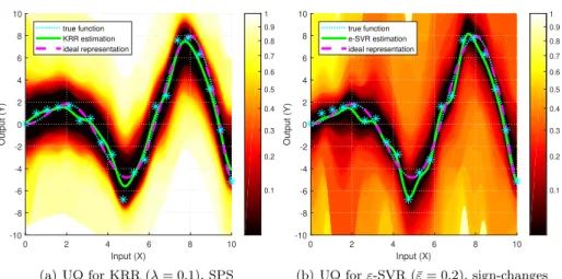
Experiments illustrating the family of (exact, non-asymptotic, distribution- free) confidence regions of KRR with Gaussian kernels and Laplacian measurement noises, and comparing the results with that of support vector regression, are shown in Figure2. The discussion of the comparison is located in Section5.3.
5.3 Uncertainty Quantification for Support Vector Regression
The previous examples were quadratic and therefore, for symmetric noises, their uncertainty could be quantified with SPS. This may be no more true if we change the applied norms. In this section we study support vector regression, particularly, ε-SVR (Hofmann et al.,2008;Sch¨olkopf and Smola,2001; Steinwart and Christ- mann,2008). A well-known advantage ofε-SVR, for example, over KRR, is that it ensures sparse representations through theε-insensitive loss function. In order to avoid confusion with the true noise vector, ε, we denote the tolerance parameter of the loss function by ¯ε. The primal objective function ofε-SVR is defined as
h(f,Dn) .
= 1
2kfk2H + c n
n
X
k=1
max{0,| hf, φ(xk)iH−yk| −ε¯}, (40) where f ∈ H,c >0, andφ(z) .
=k(z,·) is thefeature map. Function (40) can be reformulated by applying slack variables, then using standard arguments based on the Lagrangian and the Karush–Kuhn–Tucker (KKT) conditions, we arrive at the Wolfe dual ofε-SVR (Sch¨olkopf and Smola,2001), where we have to maximize
g(fα+,α−,Dn) = yT(α+−α−)−
−1
2(α+−α−)TKx(α+−α−)−ε¯(α++α−)T1, (41) subject to the (linear) constraints: α+, α− ∈ [ 0,c/n]n and (α+−α−)T1 = 0.
One can work directly with the quadratic dual objective, but then the confidence region will be constructed forα+, α−. Since,α = α+−α−, the region could be mapped to a confidence region in the space of coefficient vectors. Alternatively, one can reformulate (41) directly for coefficient vectorαas
g(fα,Dn) = yTα− 1
2αTKxα−ε¯kαk1, (42) wherek · k1 is the 1-norm. A subgradient of (42) w.r.t.αis given by
∇αg(fα,Dn) = y − Kxα − ε¯sign(α), (43) where sign(·) denotes the signum function and it is understood component-wise.
0 2 4 6 8 10 Input (X)
-10 -8 -6 -4 -2 0 2 4 6 8 10
Output (Y)
0.1 0.2 0.3 0.4 0.5 0.6 0.7 0.8 0.9 1 true function
KRR estimation ideal representation
(a) UQ for KRR (λ= 0.1), SPS
0 2 4 6 8 10
Input (X) -10
-8 -6 -4 -2 0 2 4 6 8 10
Output (Y)
0.1 0.2 0.3 0.4 0.5 0.6 0.7 0.8 0.9 1 true function
e-SVR estimation ideal representation
(b) UQ forε-SVR (¯ε= 0.2), sign-changes
Fig. 2 Exact, non-asymptotic, distribution-free confidence regions for ideal RKHS represen- tations. Parts (a) and (b) show UQ for Kernel Ridge Regression (KRR) withλ = 0.1 and ε-Support Vector Regression (ε-SVR) withc= 250 and ¯ε= 0.2, respectively. The same data was used for both regression problems, namely, the true function wasf∗(x) =xsin(x), there weren= 20 observations having i.i.d. Laplace noise with parametersµ= 0 (location) and b =1/2(scale), and Gaussian kernels were applied with σ =1/2. Part (a) was built by the Sign-Perturbed Sums (SPS) method, (29), and formula (44) was used with sign-change matri- ces for part (b). The confidence level of each color can be interpreted by using the scale bars.
The regions are increasing, i.e.,Ap⊆Aqifp≤q, thus, only the smallest levels are shown.
Then, building on the subgradient of the dual objective, i.e., (43), reference and perturbed evaluation functions can be defined, fori= 0, . . . , m−1, as
Zi(α) .
= kGi(y−Kxα)− ε¯sign(α)k2, (44) where G0 is the identity matrix and Gi is a (uniformly chosen) element of the applied compact transformation group, such as a diagonal matrix with±1 entries, for symmetric noises (or permutation matrices for exchangeable noises, etc.).
A numerical experiment illustrating the obtained family of confidence regions of theε-SVR estimate for various significance levels is shown in Figure2.
The same data sample was used for all regression models, to allow their com- parison. The noise affecting the observations was Laplacian, thus heavy-tailed.
Since the coefficient space is high-dimensional, and there is a one-to-one corre- spondence between coefficient vectors and kernel models, the confidence regions are mapped and shown in the model space, i.e., in the space of RKHS functions.
Note that it is meaningful to plot the confidence regions even for unknown input values, because the confidence regions are built for the ideal representation, which belongs to the chosen RKHS, unlike the underlying true function.
We can observe that the uncertainty of ε-SVR was higher than that of KRR, which can be explained as the price of usingε-insensitive loss. As the experiments with KLASSO show (cf. Figure3), the higher uncertainty ofε-SVR is not simply a consequence of sparse representations, as KLASSO also ensures sparsity. Naturally, the confidence regions are also influenced by the specific choice of hyper-parameters which should be taken into account when the confidence regions are compared.
5.4 Uncertainty Quantification for Kernelized LASSO
Our last example covers the LASSO (least absolute shrinkage and selection oper- ator) method, which ensures sparsity via 1-norm regularization. Let us consider the kernelized version of LASSO with objective (Wang et al.,2007):
g(fα,Dn) .
= 1
2ky−Kxαk2 + λkαk1, (45) were k · k1 is the L1 (or Manhattan) norm. Though, function (45) cannot be written askz − Φαk2, the proposed framework, i.e., construction (17)-(18), can still be applied. A sub-gradient of the KLASSO objective (45) is given by
∇αg(fα,Dn) = Kx(Kxα−y) +λsign(α), (46) where the sign(·) function is applied component-wise. Then, using the construction of (17)-(18), the reference and perturbed functions can be defined as
Z0(α) .
=kKx(Kxα−y) +λsign(α)k2, (47) Zi(α) .
=kKxGi(Kxα−y) +λsign(α)k2, (48) were{Gi}are from a suitable transformation group, e.g., diagonal matrices with Rademacher random variables as diagonal elements for symmetric noises.
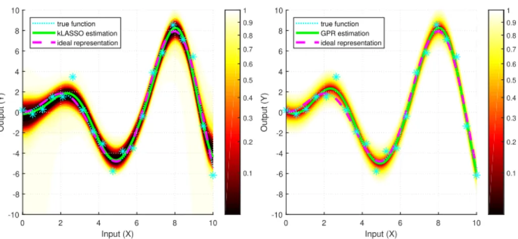
Numerical experiments illustrating the confidence regions we get for KLASSO are presented in Figure 3. The figure also presents the confidence regions con- structed by applying the standard Gaussian Process (GP) regression with esti- mated parameters. Note that the GP confidence regions are only approximate, namely, they do not come with strict finite-sample guarantees unless the noise is indeed Gaussian. Moreover, during our experiment the noise had a Laplace distribution, which has a heavier tail than Gaussians, therefore even if the true covariance of the noise was known, the confidence regions of GP regression would underestimate the uncertainty of the estimate (would be too optimistic), while the confidence regions of our framework are always non-conservative, independently of the particular distribution of the noise, assuming it has the necessary invariance.
Also note that for our method the noises can even have different (marginal) distributions for each input. Therefore, even though the confidence regions gener- ated by GP are smaller than the ones our framework produces, the GP regions are imprecise and underestimate the uncertainty of the model, while ours come with strict finite-sample guarantees for a broad class of noises (e.g., symmetric ones).
6 Conclusions
In this paper we addressed the problem of quantifying theuncertainty of kernel estimates by using minimal distributional assumptions. The main aim was to mea- sure the uncertainty of finding the (noise-free)ideal representationof the underly- ing (hidden) function at the available inputs. By building on recent developments in finite-sample system identification, we proposed a method that deliversexact, distribution-freeconfidence regions with strongfinite-sample guarantees, based on the knowledge of some mild regularity of the measurement noises. The standard
0 2 4 6 8 10 Input (X)
-10 -8 -6 -4 -2 0 2 4 6 8 10
Output (Y)
0.1 0.2 0.3 0.4 0.5 0.6 0.7 0.8 0.9 1 true function
kLASSO estimation ideal representation
(a) UQ for KLASSO with Gaussian kernel
0 2 4 6 8 10
Input (X) -10
-8 -6 -4 -2 0 2 4 6 8 10
Output (Y)
0.1 0.2 0.3 0.4 0.5 0.6 0.7 0.8 0.9 1 true function
GPR estimation ideal representation
(b) UQ with Gaussian Process Regression
Fig. 3 Exact, non-asymptotic, distribution-free confidence regions for ideal RKHS representa- tions obtained using our framework and approximate confidence regions obtained by Gaussian Process (GP) regression (Rasmussen and Williams,2006). Part (a) shows UQ for Kernelized LASSO with λ = 1, and part (b) shows UQ with GP. The applied transformations were sign-change matrices. The same data was used for both regression problems, namely, the true function wasf∗(x) =xsin(x), there weren= 20 observations having i.i.d. Laplace noise with parametersµ= 0 (location) andb=1/2(scale), and Gaussian kernels were applied withσ= 1.
The confidence level of each color can be interpreted by using the scale bars. The confidence regions are increasing, i.e.,Ap⊆Aqifp≤q, therefore, only the smallest levels are shown.
examples of such regularities areexchangeableorsymmetricnoise terms. Note that either of these properties in itself is sufficient for the theory to be applicable.
The needed statistical assumptions are very mild, as for example, no particular (parametric) family of distributions was assumed, no moment assumptions were made (the noises can be heavy-tailed, and may even have infinite variances); more- over, for the case of symmetric noises, it is allowed that each noise term affecting the observations has a different distribution, i.e., the noise can benonstationary.
The core idea of the approach is to evaluate the uncertainty of the estimate byperturbing the residualsin thegradientof the objective function. The norms of the (potentially weighted) perturbed gradients are then compared to that of the unperturbed one, and arank testis applied for the construction of the region.
The proposed method was also demonstrated on specific examples of ker- nel methods. Particularly, we showed how to construct exact, non-asymptotic, distribution-free confidence regions for least-squares support vector classification, kernel ridge regression, support vector regression and kernelized LASSO.
Severalnumerical experimentswere presented, as well, demonstrating that the method provides meaningful regions even forheavy-tailed(e.g., Laplacian) noises.
The figures illustrate whole families of confidence regions for various standard kernel estimates. Ellipsoidal outer approximations are also shown for LS-SVC.
Additionally, the method was compared to Gaussian Process (GP) regression, and it was found that although the (approximate) GP confidence regions are smaller in general than our (exact) confidence sets, but the GP regions are typically imprecise and they underestimate the real uncertainty, e.g., if the noises are heavy-tailed.
Our approach to build non-asymptotic, distribution-free, non-conservative con- fidence regions for kernel methods can be a promising alternative to existing con- structions, which arch-typically either build on strong distributional assumptions or on asymptotic theories or only bound the error between the true and empirical risks. As our approach explicitly builds on the constructions of the underlying kernel methods, it can provide new insights on how the specific methods influ- ence the uncertainty of the estimates, and therefore, besides being vital for risk management, it also has the potential to inspire refinements or new constructions.
There are several open questions about the framework which can facilitate future research directions. For example, finding efficientouter-approximationsfor cases when the objective function is not convex quadratic should be addressed. Also the consistencyof the method should be studied to see whether the uncertainty decreases as the sample size tends to infinity. Finally, it would be interesting, as well, to extend the method to (stochastic) dynamical systemsand to formally analyze thesize and shapeof the constructed regions in a finite-sample setting.
Acknowledgements This research was supported by the National Research, Development and Innovation Office (NKFIH), grant numbers ED 18-2-2018-0006, 2018-1.2.1-NKP-00008 and KH 17 125698. The authors are grateful to Algo Car`e for the valuable discussions.
A. Additional Numerical Experiments
In this appendix we provide additional numerical experiments supporting the pre- sented framework. The effects of variousmeasurement noises,kernel functionsand sample sizeson the obtained (families of) exact, non-asymptotic, distribution-free confidence regions were studied. The true function was always f∗(x) = xsin(x) and the inputs were chosen equidistantly from [ 0,10 ]. The regions were evaluated by the same methodology (Monte Carlo simulations) as in Section5.
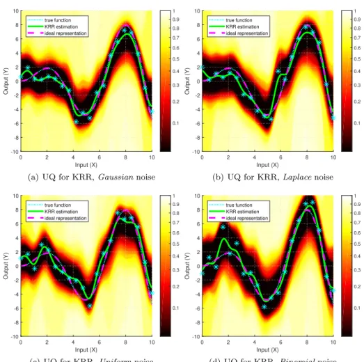
A.1 Various Noise Distributions
First, we investigated how the distribution of the noise affects the regions. Par- ticularly, we applied Gaussian, Laplacian, Uniform and Binomial noises on the outputs of the true function and built the regions for Kernel Ridge Regression (KRR). All noises had zero mean (for the Binomial case the theoretical mean was subtracted from the generated noises), and the parameters of the distributions were set in a way to ensure that all of their variances were the same (i.e., one).
Figure4illustrates the obtained families of confidence sets. It can be observed that their shapes and sizes show only small fluctuations indicating that the par- ticular choice of the distribution has a limited effect on the confidence regions (assuming it has zero expectation and we keep the variance of the noise fixed).
A.2 Different Kernel Functions
Next, the effect of the applied kernel was studied. Figure5illustrates UQ for ker- nelized LASSO withGaussian,Laplacian,truncated parabolic(k(x, y) = max{1−