Increasing RSSI Localization Accuracy with Distance Reference Anchor in Wireless Sensor Networks
Ugur Bekcibasi
1, Mahmut Tenruh
21 Mugla S. K. University, Faculty of Technology, Department of Information Technology, 48000 Mugla, Turkey; e-mail: ugur@mu.edu.tr
2 Mugla S. K. University, Department of Electrical and Electronics Engineering, 48000 Mugla, Turkey; e-mail: tmahmut@mu.edu.tr
Abstract: Localization is a prominent application and research area in Wireless Sensor Networks. Various research studies have been carried out on localization techniques and algorithms in order to improve localization accuracy. Received signal strength indicator is a parameter, which has been widely used in localization algorithms in many research studies. There are several environmental and other factors that affect the localization accuracy and reliability. This study introduces a new technique to increase the localization accuracy by employing a dynamic distance reference anchor method. In order to investigate the performance improvement obtained with the proposed technique, simulation models have been developed, and results have been analyzed. The simulation results show that considerable improvement in localization accuracy can be achieved with the proposed model.
Keywords: RSSI; Wireless Sensor Networks; WSN Localization
1 Introduction
The wireless sensor network (WSN) concept was first emerged in early 1980s.
Since 1990s, it has been an important research area due to the progresses in micro electro-mechanic systems (MEMS) and wireless communication techniques.
Although wireless sensor networks were initially used mainly in military applications, they have also been used in various applications in different areas.
Depending on the hardware configurations, WSNs can be used to acquire data about various physical properties such as temperature, humidity, light, pressure, movement, soil composition, noise level, existence, weight, dimensions, velocity, direction, location [1]. WSNs can be deployed in various environments, where wired networks are impossible or impractical to deploy.
Due to their features such as reliability, flexibility, self-organization, and ease of deployment, WSNs have a wide range of present and possible future application areas. In the environment they are used, WSNs can interactively acquire data.
WSNs have been an attractive research area, and therefore, experienced a rapid development, and found a variety of application areas such as military applications (C4ISRT) [2], environmental detection and monitoring [3], disaster prevention and rescue, medical applications, body network [4], smart house systems [5], smart fields [6], the cricket location support system [7], cooperative localization and tracking with a camera-based WSN [5] and resources tracking at building construction sites [8].
One of the important application areas of WSN is localization, on which several research studies have been realized, and several techniques have been developed.
The common problem in localization is the additional hardware requirement and power consumption. The additional hardware and the resulting increased power consumption do not fit the energy-efficient WSN concept. The most power consuming component in a WSN node is the communication unit. Therefore, several research studies also investigate the ways to save energy. In addition, the environmental conditions make further studies necessary for better performance localization. Several studies investigated localization in WSNs with different techniques such as range-based [9], range-free [10], use of anchor and recursive solutions [11], MDS-based [12], centralized-distributed [9], mobile assisted [13], and cluster-based [14, 15].
In this study, a new method which uses a fourth anchor node as a measurement reference in received signal strength indication (RSSI) technique is introduced. In order to investigate the performance of the introduced method, simulation models have been designed and the results have been evaluated. According to the simulation results, the new method provides considerable performance improvement in localization.
The rest of the paper is organized as follows. In Section 2, a review of localization techniques in WSNs is provided. In this section, distance estimation, position computation, and localization algorithms are investigated. In addition, the factors affecting RSSI measurement and accuracy are also included. In Section 3, the simulation model is introduced. In order to compare performance improvements in localization, a second simulation model with the traditional method has also been designed. In Section 4, the simulation results are investigated and performance analysis is realized. The simulation results for the new model and traditional model are compared in graphs and tables. Finally, Section 5 provides the concluding remarks for the paper.
2 Localization In Wireless Sensor Networks
Localization is one of the main application areas in wireless sensor networks.
Localization can be used in various applications such as determining coverage area of WSN, monitoring location changes, geographical area-based routing, and location directory services. Wireless sensor networks may contain hundreds of nodes; where it may cause a high cost to use the global positioning system (GPS) for each node [16]. Therefore, as stated in the study by Sheu et al (2008), such a solution is not suggested. In addition, as GPS receivers require relatively high energy, it is not suitable for the fundamental idea of energy-efficient WSNs.
In applications where only local location information is sufficient, there is no need for GPS. In this case, sensor nodes with known locations, called anchors, are used to determine the local coordinates of other nodes. In applications requiring global localization information, anchor nodes with GPS can be used, or anchor nodes can be located at known coordinates [16].
Several studies suggest different measurement techniques and localization algorithms. WSN localization techniques can be classified into several categories.
The localization process is generally comprised of three phases. These are distance estimation; position computation; and localization algorithm [17].
Distance Estimation: In the distance estimation phase, the relative distances between the nodes are estimated via the measurement techniques. The four common measurement techniques can be classified as the angle of arrival (AoA), time of arrival (ToA), time difference of arrival (TDoA), and received signal strength indicator (RSSI). These are also known as range-based localization techniques.
Position computation: The coordinates of a node are calculated via the range or connectivity information. The main techniques used in localization are lateration, multilateration, and angulation. The lateration technique is used to compute the location of a node with the distance measurements obtained by three anchor nodes [9]. With the range information obtained by four anchors, it is also possible to realize three-dimensional localization. Trilateration is the process of lateration realized with three anchors. Lateration with more than three anchors is called multilateration. In angulation or triangulation method, the localization is computed based on the angle information obtained at least via three anchor nodes. In this method, the computation is realized by the node itself with the AoA information using trigonometric solutions [9].
Localization algorithms: WSN localization algorithms can be classified into several categories such as: single-hop or multi-hop based on the node connectivity and topology; range-based or range-free based on the dependency of the range measurement; distributed or centralized position computation [17].
Determining the distance between two communicating nodes is essential for localization in wireless sensor networks. In range-based algorithms, localization is realized with the distance information between two nodes obtained via several techniques such as angle of signal arrival, time difference of signal arrival, and received signal strength [9]. Since range-based algorithms require measurement at least via one anchor node, these techniques are also known as one-hop techniques [18].
2.1 Localization with Received Signal Strength Indication
In this study, the RSSI technique is used as the distance estimation method. The RSSI technique is based on the received signal strength indicator to estimate the distance between neighboring nodes. In free-space, the RSSI value is inversely proportional to the squared distance between the transmitter and the receiver. The radio signals attenuate with the increase of the distance. The propagation of the radio signals may be affected by reflection, diffraction, and scattering. Especially in indoor environments, such effects may impact the measurement accuracy.
Therefore, this technique is more suitable for outdoor, rather than indoor applications.
This technique has the advantage of requiring no additional hardware since the RSSI feature exists in most wireless devices, and there is no significant impact on the local power consumption [11].
RSSI is affected from some factors that cause localization errors and reduce accuracy. These errors can be classified into two groups as environmental and device errors. Environmental errors are caused due to wireless communication channel. The causes are usually multi path, shadowing effect, and interference from other RF sources. Device errors are usually caused due to calibration errors, and the important issue here is to keep constant transmit power even under the circumstances of device differences and depleting batteries.
Signal samples, even with the same transmit power, show some standard deviations due to atmospheric conditions. Temperature, for example, has a little effect on a signal. However, rain can affect the signal considerably. Especially, in localization based on the received signal strength method, this will cause less accuracy and reliability [19].
2.2 Localization Process in the Introduced Model
In order to realize the localization with the introduced reference anchor node, which provides the dynamic coefficient for more accurate distance measurements, the following equations are used [20]. First, the RSSI value can be calculated with the Equation 1:
) ) log(
. . 10
( d A
RSSI (1)
where RSSI is the Received Signal Strength indicator measured by the receiving anchor node. In this case, the receiving node is the base node, and the sending node is the reference anchor node. η is the coefficient depending on the environmental conditions (which may change between 1.6 and 6). d is the distance between the receiving anchor node and the sending node, in this case, the base node and reference anchor node respectively, where the distance is already known.
A is the absolute value of RSSI for the distance of 1 m. given by the producer, for example, A = -51 dBm for CC2420 radio communication chip by the TI.
Then, in order to compute the coefficient (η), also recomputed in every localization process according to the changing environmental conditions, the following equation is used:
) log 10
( d
A RSSi
(2)
The coefficient η is computed with the RSSI value obtained from the reference anchor by the base node. As the distance to the reference anchor is already known, this distance is used in the equation to compute the η coefficient. Then, the computed η is used to estimate more accurate distance values with the RSSI values transmitted by other three anchor nodes. In order to compute the distances of the anchor nodes to the node to be localized, the following equation is used.
10
( 10 )
d
A RSSi
(3)
After the distances of the anchor nodes to the localized node are computed by the base node, the trilateration method is applied to estimate the exact location. As this localization process is realized with the dynamically computed η coefficient according to the changing environmental conditions for each individual localization process, more accurate localization estimates are expected.
3 Material And Method
In this study, the RSSI method is applied in the simulation models. Due to the low computation capacity on WSN nodes, and the necessity to save energy, relatively low mathematical computation requiring circular localization technique is applied.
The OMNEST 4.1 simulation software is used to develop the system models.
3.1 Simulation Model
The simulation model designed in this study includes mobile, reference, and anchor nodes. In the simulation, a square area with the dimensions of 100m x 100m has been modeled. In the model, a moving node continuously transmits existing information, and the anchor nodes located at the four corners of the area relay the signal strength information of the moving node to the base anchor node.
The base anchor node computes the location of moving node. The location information produced in this process can be monitored with a computer connected to the base anchor. The simulation model components and the RSSI data flow can be seen in Figure 1.
Figure 1
Simulation model functionality diagram
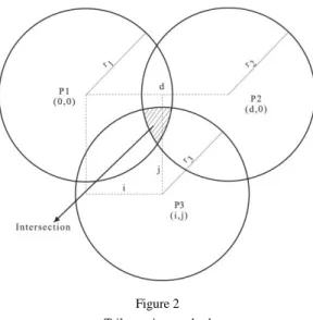
In this study, trilateration method is applied to compute localization. This is the method which requires the least computing power to find the intersection of three circles. Due to its computational simplicity, this method is suitable for the microcontroller in a WSN node. The trilateration method is depicted in Figure 2.
Figure 2 Trilateration method
This method finds the localization coordinates via intersection area of three circles with known radiuses on a coordinate plane by simplified equations. The equation group used in the method to compute the coordinates can be seen in Equation 4.
2 2 2
1 2
2 2 2 2 2
1 3
2 2 2
1
2
2
r r d
x d
r r x x i j
y j
z r x y
(4)
A distance of 100 m between two adjacent nodes is usually described as the coverage distance of a node with 10 mW transmit power under free space and direct line of sight conditions. Since the model is considered with two dimensions, the third dimension z is not required and excluded from computation.
The system model shown in Figure 3 includes four anchor nodes, where one node is added as a reference anchor to the traditional three anchor method.
Figure 3 Four anchor measurement
In order to evaluate the performance improvement achieved with the introduced reference-anchor model, a traditional three anchor model has also been designed as seen in Figure 4.
In the proposed model, the moving node realizes periodic transmissions, and the signal strength indication (RSSI) information is produced separately at each receiving anchor node. Each anchor node transmits its RSSI information to the base node. At the base node, first three RSSI values are used to find coordinates of the moving node. Although the trilateration method is used for localization, a coefficient value obtained from the fourth anchor node is also used in localization process. The main contribution of the introduced model is that the fourth anchor node is used as a distance reference. The base node also acts as a dynamic distance coefficient producer. Since the fixed distance between the base station and the reference node is already known, the received signal strength from the reference node can be used to produce a distance coefficient at the base node. The coefficient value is determined dynamically according to changing environmental effects, such as atmospheric conditions, for every measurement. In this way, measurement errors originating from environmental effects, which result in varying RSSI values, can be eliminated considerably.
Figure 4 Three anchor measurement
The base station receives the RSSI values of the moving node from any three anchor nodes, and the fourth signal received from the last anchor is used to produce its RSSI value, which also determines the coefficient to be used in localization process. It can be argued that the coefficient value can also be produced from the received signal strength of an anchor node in the traditional three anchor model. In this concept, the fourth anchor node means an additional cost to the system. However, the fourth node also provides some advantages, such as more coverage and fault tolerance. If the moving node is outside the coverage area of one anchor, the other three anchors may still provide enough coverage.
Especially in the case of one anchor node failure, the remaining three anchor nodes will still continue to function, and therefore, the system will also have fault tolerance. In this case, the coefficient is still produced by the base node with the last received signal of the three remaining nodes.
The main idea in this study is to investigate the performance improvement obtained with the reference anchor model against the traditional three anchor model. Since the focus is on the evaluation of the improvement provided by the new method, both model nodes are considered to be under the same environmental conditions. Performance improvement is based on the dynamically computed η environmental coefficient, in contrast to the constant η coefficient used in the traditional model. In order to evaluate the performance improvement, only the measurements with different fixed locations are covered. However, similar results
can be expected for moving nodes since the measurements are considered to be realized under the same conditions for both models. Figure 5 illustrates the simplified flow chart for the functionality of the system.
Figure 5
Simplified functionality flow chart diagram
4 Simulation Results And Performance Analysis
The simulation models have been operated with three different distance scenarios.
In the first scenario, the moving node is located at the center of the area having (50;50) coordinates which have equal distances to all anchor nodes. In the second scenario, the moving node is located at the (28;37) coordinates which have different distances to the anchor nodes. The third scenario has the coordinate values of (75;50) for the moving node. These three different coordinates have been applied to both the traditional three anchor model, and the introduced fourth reference anchor model. Figure 6 and Figure 7 show the simulation models of three anchor nodes, and four anchor nodes respectively. These models aim to present the performance improvement obtained with the fourth node used as the measurement reference anchor. In the introduced model, before applying the trilateration method, the dynamic distance coefficient is used for scaling.
In the simulation studies, the localization processes have been realized repeatedly 100 times for all three coordinates. In every localization process, the coordinate values are kept constant in order to obtain the distribution of localization values for one point.
Figure 6
Simulation model for trilateration
Figure 7
Simulation model for reference anchor
Simulation results for the coordinates of (50;50) can be seen in Figure 8. In this figure, the results for the both models are shown together for better comparison purposes. Table 1 provides the statistical minimum, maximum, average, and standard deviation values of the obtained measurements for both models. From the figure and table, it can be seen that although the traditional three anchor model provides a very close average value to the real point for the x axis, the y axis has a measurement error of about 2.88 meters. On the other hand, although the standard deviation value is slightly higher for the reference anchor model in y axis, the average values almost reach the exact coordinate values with only about 58.9 cm, and 61.9 cm differences on the x and y axes respectively. On the basis of the minimum and maximum measured values, although the y axis has more minimum measurement error for the introduced model, the other measurement values show better results. Moreover, as can be seen in Figure 8, the exact location coordinates are located in the center of the measured values with the reference anchor model.
On the other hand, the traditional model values are scattered around a center beyond the exact location. These results show that the introduced new model produces better measurement results and has a higher performance over the traditional three anchor model.
Figure 8
Measurement result for 50-50 coordinates
Table 1
Statiscial values for 50-50 coordinates
(50;50) 3 anchor Reference anchor
x y x y
Mean 49.240 52.878 50.589 50.619
Maximum 62.572 60.936 60.289 60.106
Minimum 38.097 45.359 40.347 40.251
Standard Dev. 6.1650 3.362 4.905 4.5923
The simulation results of the both models for the (28;37) coordinates are also shown together in Figure 9. This location is chosen to be closer to the anchor node A1. As can be seen from the figure, for this location, the area of some scattered measurement results of the both models overlap. However, the exact location point is again in the center of the results obtained for the reference anchor model.
Table 2 also shows the statistical results for both models. According to these results, it can be seen that the average measurement results for the reference anchor model show much better performance with the measurement differences in the order of centimeters (x: 0.073 m, y: 0.261 m), while the three anchor model produces measurement errors in the order of meters (x: 6.482 m, y: 3.199 m).
From the point of maximum and minimum measurement values, and standard deviation values, the proposed model mainly produces better results. These results show that the reference anchor model provides improved performance for also this location.
Figure 9
Measurement result for 28-37 coordinates
Table 2
Statiscial values for 28-37 coordinates
(28;37) 3 anchor Reference anchor
x y x y
Mean 21.517 33.800 28.073 37.261
Maximum 32.240 47.457 35.852 42.079
Minimum 10.128 18.346 16.510 28.925
Standard Dev. 5.726 7.035 4.276 3.263
Figure 10
Measurement result for 75-50 coordinates
Table 3
Statiscial values for 75-50 coordinates
(75;50)
3 anchor Reference anchor
x y x y
Mean 82.510 54.105 75.765 50.624
Maximum 97.675 63.725 85.964 63.694
Minimum 69.729 44.505 64.390 35.498
Standard Dev. 6.803 4.298 5.4186 6.109
Finally, the model performances are compared for the location coordinates (75;50), and the results are shown in Figure 10 and Table 3. From the figure, once more, it can be seen that the exact location point is in the center of distributed values obtained for the proposed model. The table shows that the average measurement values for the proposed model almost give the exact location coordinates with differences only in the order of centimeters (x: 76.5 cm, y: 62.4 cm), while the traditional model presents 7.51 meters, and 4.1 meters errors on the x and y axes respectively. From these results, it can be seen that the new model provides considerably better measurement performances.
Figure 11 shows all the statistical results together for comparison purposes. As seen in this figure, in all three cases the coordinates of exact points are located on the central point of value lines obtained for the proposed model. In some studies, averaging a few consequent measurements is used to obtain closer values to the exact location. From the simulation results, it is clear that a simple averaging process will produce very close values to the exact location with the proposed system.
Figure 11 Measurement graphs
Conclusions
In this study, a new technique in RSSI localization method for wireless sensor networks has been introduced. The technique proposes a distance reference anchor node which provides a dynamic correction coefficient for every measurement. The distance reference anchor node provides a continuous feedback about the RSSI changes due to environmental effects. The base node uses the RSSI information from the reference anchor node to produce a correction coefficient. The coefficient is applied to the trilateration computation to find the location of a moving node. In this study, the reference node is arranged as a fourth anchor which is an additional node to the traditional trilateration model, which needs three anchor nodes for localization process. It has been explained that although adding a fourth anchor node to the system may cause an additional cost, it provides some benefits, such as more coverage area and fault tolerance.
In order to evaluate the performance improvement achieved with the proposed model, a three node traditional localization model has also been developed. Both models have been simulated for three different locations and statistical results have been obtained. The simulation results have been evaluated and the performances of the both models have been compared in graphs and tables. The simulation results showed that the proposed model with the reference anchor produced better measurement results than the traditional localization model. This
is because the proposed technique introduces the use of a correction coefficient in the localization process. The coefficient is produced dynamically according to the environmental conditions. As distance correction is realized dynamically for every localization process, the localization error is kept to a minimum. Therefore, environmental effects, such as atmospheric conditions, causing distance measurement errors, are eliminated considerably, and better localization results in WSN systems can be achieved. From the simulation results obtained in this study, it can be concluded that the proposed new technique provides considerable performance improvement in RSSI localization.
References
[1] Akyildiz, I.: Wireless Sensor Networks: a Survey, Computer Networks, 38, 2002, pp. 393-422
[2] Diamond S. M., Ceruti M. G.: Application of Wireless Sensor Network to Military Information Integration, in: 5th IEEE International Conference on Industrial Informatics, IEEE, 2007, pp. 317-322
[3] Ma R. H., Wang Y. H., Lee C. Y.: Wireless Remote Weather Monitoring System Based on MEMS Technologies., Sensors, 11, 2011, pp. 2715-2727 [4] Yang G. Z., Yacoub M.: Body Sensor Networks, 2006, Springer, London [5] Sanchez-Matamoros J. M., J. Martinez de Dios, Ollero A.: Cooperative
Localization and Tracking with a Camera-based WSN, 2009 IEEE International Conference on Mechatronics, IEEE, 2009, pp. 1-6
[6] Want R., Hopper A., Falcao V., Gibbons J.: The Active Badge Location System, ACM Transactions on Information Systems 10, 1992, pp. 91-102 [7] Priyantha N. B., Chakraborty A., Balakrishnan H.: The Cricket Location
Support System, 6th ACM International Conference on Mobile Computing and Networking, 2000, Boston, Massachusetts, USA
[8] Shen X., Chen W., Lu M.: Wireless Sensor Networks for Resources Tracking at Building Construction Sites, Tsinghua Science & Technology 13, 2008, pp. 78-83
[9] Mao G., Fidan B., Anderson B.: Wireless Sensor Network Localization Techniques, Computer Networks, 51, 2007, pp. 2529-2553
[10] Bulusu N., Heidemann J., Estrin D.: GPS Less Low-Cost Outdoor Localization for Very Small Devices, IEEE Personal Communications, 7, 2000, pp. 28-34
[11] Wang C., Xiao L.: Locating Sensors in Concave Areas, IEEE INFOCOM 2006, 25th IEEE Int. Conf. on Computer Communications, 2006, pp. 1-12 [12] Ji X., Zha H.: Sensor Positioning in Wireless Ad-Hoc Sensor Networks
using Multidimensional Scaling, INFOCOM 2004, 4, IEEE, 2004, pp.
2652-2661
[13] Priyantha N., Balakrishnan H., Demaine E., Teller S.: Mobile-assisted Localization in Wireless Sensor Networks, 24th Annual Joint Conference of the IEEE Computer and Communications Soc., 1, IEEE, 2005, pp. 172-183 [14] Medidi M.: Cluster-based Localization in Wireless Sensor Networks,
Proceedings of SPIE, 6248, SPIE, 2006, pp. 62480J-62480J-9
[15] Sheng X., Hu Y. H.: Collaborative Source Localization in Wireless Sensor Network System, IEEE Globecom, 2003
[16] Sheu J. P., Member S., Chen P. C., Hsu C. S.: A Distributed Localization Scheme for Wireless Sensor Networks with Improved Grid-Scan and Vector-based Refinement, IEEE Transactions on Mobile Computing 7, 2008, pp. 1110-1123
[17] Bal M., Liu M., Shen W.: H. Ghenniwa, Localization in Cooperative Wireless Sensor Networks: A Review, 2009, pp. 438-443
[18] Hu L., Evans D.: Localization for Mobile Sensor Networks, MobiCom '04, October, ACM Press, New York, USA, 2004, p. 45
[19] Clark M. P.: Radio Propagation, System Range, Reliability and Availability, Wireless Access Networks: Fixed Wireless Access and WLL Networks - Design and Operation, 2000, pp. 115-139
[20] Wang X., Bischoff O., Laur R., Paul S.: Localization in Wireless Ad-hoc Sensor Networks using Multilateration with RSSI for Logistic Applications, Procedia Chemistry 1, 2009, pp. 461-464