Detection of 2x2 MIMO signals
I. IntroductIon
II. themodel
SEPTEMBER 2020 • VOLUME XII • NUMBER 3 24
INFOCOMMUNICATIONS JOURNAL
János Ladvánszky1
Detection of 2x2 MIMO signals
1 Formerly with Ericsson Hungary, Budapest, Hungary.
(e-mail: Ladvanszky55@t-online.hu)
Abstract— In this paper, we investigate synchronization and equalization of 2 x 2 MIMO signals. We make a step further than that is described in our patent. In the patent, 3 PLLs and a four- channel adaptive filter was needed. Here we decrease the number of PLLs to two and use an adaptive filter of only two channels.
In addition to that, we shortly introduce the filter method and the FFT method as well, for synchronization. False detection cancellation is also mentioned. The so-called 1-bit technique has been compared to our method. After briefly introducing the ideas, detailed Matlab or AWR analyses follow. Input data are real measurements, so the analyses serve also as experimental verifications. We take a glimpse on higher order MIMO and higher order modulations as well.
Index Terms—MIMO, synchronization, equalization, false de- tection cancellation
DOI: 10.13164/re.2019.0001 CATEGORY (E.G. CIRCUITS)
Detection of 2x2 MIMO signals
János LADVÁNSZKY
11Formerly with Ericsson Hungary, 1117 Budapest, Magyar tudósok körútja 11, Hungary
Submitted January 1, 2019/ Accepted January 2, 2019
Abstract. In this paper, we investigate synchronization and equalization of 2 x 2 MIMO signals. We make a step further than that is described in our patent. In the patent, 3 PLLs and a four-channel adaptive filter was needed. Here we decrease the number of PLLs to two and use an adaptive filter of only two channels. In addition to that, we shortly introduce the filter method and the FFT method as well, for synchronization. False detection cancellation is also mentioned. The so-called 1-bit technique has been compared to our method. After briefly introducing the ideas, detailed Matlab or AWR analyses follow. Input data are real measurements, so the analyses serve also as experimental verifications. We take a glimpse on higher order MIMO and higher order modulations as well.
Indexing terms
MIMO, synchronization, equalization, false detection cancellation
1.Introduction
The 2 x 2 MIMO (Multiple Input Multiple Output) concept is shown in Fig. 1. The core of the idea is that 2-2 transmitter and receiver antennas can provide better system properties than two transmitter-receiver antenna pairs separately.
Fig. 1.The 2 x 2 MIMO concept. From d and the operation frequency, h is determined
For achieving this, a 90° difference in electrical length is needed between each transmitter antenna to the two receiver antennas.
Both receiver antennas receive two signals shifted in time. If the modulation is 4QAM, then based on the
properties of the signal, the two transmitted information can be separated. For separation, estimated receiver frequencies should be known. Finding the exact receiver frequencies (synchronization) and the reconstruction of the constellation diagrams (channel equalization) can be realized by three PLLs and a four-channel adaptive filter [2].
In this paper, our more recent solution will be described that requires only two PLLs and a two-channel adaptive filter. The best overview about MIMO is found in [1]. In [2], our patent about MIMO is described. In [3], use of more than 4 antennas are investigated. Higher order modulations than 4QAM are discussed in [4]. DSc dissertation of the author, including a thesis about MIMO, is obtained in [5].
2. The model
The model of a 2 x 2 MIMO communication system is shown in Fig. 2.
Fig. 2. Model of a 2 x 2 MIMO communication system. 𝑥𝑥, 𝑟𝑟 denotes the column matrices of transmitted and received
signals, respectively
According to Fig. 2, an equalizer is applied for the receiver signal to reconstruct the transmitted signal.
𝑟𝑟 = [𝑎𝑎 𝑏𝑏𝑏𝑏 𝑎𝑎] 𝑥𝑥 (1)
Eq. (1) describes the antenna system. In ideal case,
𝑎𝑎 = 1 (2)
𝑏𝑏 = 𝑒𝑒−𝑗𝑗𝑗𝑗/2= −𝑗𝑗 (3)
And the reconstruction:
𝑥𝑥̂ = [𝑎𝑎′ 𝑏𝑏′
𝑏𝑏′ 𝑎𝑎′]−1𝑟𝑟 (4)
Our goal is
|𝑥𝑥̂ − 𝑥𝑥| = 𝑚𝑚𝑚𝑚𝑚𝑚. (5)
And the minimum in Eq. (5) is zero if
𝑎𝑎′= 𝑎𝑎 (6)
1
DOI: 10.13164/re.2019.0001 CATEGORY (E.G. CIRCUITS)
Detection of 2x2 MIMO signals
János LADVÁNSZKY
11Formerly with Ericsson Hungary, 1117 Budapest, Magyar tudósok körútja 11, Hungary
Submitted January 1, 2019/ Accepted January 2, 2019
Abstract. In this paper, we investigate synchronization and equalization of 2 x 2 MIMO signals. We make a step further than that is described in our patent. In the patent, 3 PLLs and a four-channel adaptive filter was needed. Here we decrease the number of PLLs to two and use an adaptive filter of only two channels. In addition to that, we shortly introduce the filter method and the FFT method as well, for synchronization. False detection cancellation is also mentioned. The so-called 1-bit technique has been compared to our method. After briefly introducing the ideas, detailed Matlab or AWR analyses follow. Input data are real measurements, so the analyses serve also as experimental verifications. We take a glimpse on higher order MIMO and higher order modulations as well.
Indexing terms
MIMO, synchronization, equalization, false detection cancellation
1.Introduction
The 2 x 2 MIMO (Multiple Input Multiple Output) concept is shown in Fig. 1. The core of the idea is that 2-2 transmitter and receiver antennas can provide better system properties than two transmitter-receiver antenna pairs separately.
Fig. 1.The 2 x 2 MIMO concept. From d and the operation frequency, h is determined
For achieving this, a 90° difference in electrical length is needed between each transmitter antenna to the two receiver antennas.
Both receiver antennas receive two signals shifted in time. If the modulation is 4QAM, then based on the
properties of the signal, the two transmitted information can be separated. For separation, estimated receiver frequencies should be known. Finding the exact receiver frequencies (synchronization) and the reconstruction of the constellation diagrams (channel equalization) can be realized by three PLLs and a four-channel adaptive filter [2].
In this paper, our more recent solution will be described that requires only two PLLs and a two-channel adaptive filter. The best overview about MIMO is found in [1]. In [2], our patent about MIMO is described. In [3], use of more than 4 antennas are investigated. Higher order modulations than 4QAM are discussed in [4]. DSc dissertation of the author, including a thesis about MIMO, is obtained in [5].
2. The model
The model of a 2 x 2 MIMO communication system is shown in Fig. 2.
Fig. 2. Model of a 2 x 2 MIMO communication system. 𝑥𝑥, 𝑟𝑟 denotes the column matrices of transmitted and received
signals, respectively
According to Fig. 2, an equalizer is applied for the receiver signal to reconstruct the transmitted signal.
𝑟𝑟 = [𝑎𝑎 𝑏𝑏𝑏𝑏 𝑎𝑎] 𝑥𝑥 (1)
Eq. (1) describes the antenna system. In ideal case,
𝑎𝑎 = 1 (2)
𝑏𝑏 = 𝑒𝑒−𝑗𝑗𝑗𝑗/2= −𝑗𝑗 (3)
And the reconstruction:
𝑥𝑥̂ = [𝑎𝑎′ 𝑏𝑏′
𝑏𝑏′ 𝑎𝑎′]−1𝑟𝑟 (4)
Our goal is
|𝑥𝑥̂ − 𝑥𝑥| = 𝑚𝑚𝑚𝑚𝑚𝑚. (5)
And the minimum in Eq. (5) is zero if
𝑎𝑎′= 𝑎𝑎 (6)
DOI: 10.13164/re.2019.0001 CATEGORY (E.G. CIRCUITS)
Detection of 2x2 MIMO signals
János LADVÁNSZKY
11Formerly with Ericsson Hungary, 1117 Budapest, Magyar tudósok körútja 11, Hungary
Submitted January 1, 2019/ Accepted January 2, 2019
Abstract. In this paper, we investigate synchronization and equalization of 2 x 2 MIMO signals. We make a step further than that is described in our patent. In the patent, 3 PLLs and a four-channel adaptive filter was needed. Here we decrease the number of PLLs to two and use an adaptive filter of only two channels. In addition to that, we shortly introduce the filter method and the FFT method as well, for synchronization. False detection cancellation is also mentioned. The so-called 1-bit technique has been compared to our method. After briefly introducing the ideas, detailed Matlab or AWR analyses follow. Input data are real measurements, so the analyses serve also as experimental verifications. We take a glimpse on higher order MIMO and higher order modulations as well.
Indexing terms
MIMO, synchronization, equalization, false detection cancellation
1.Introduction
The 2 x 2 MIMO (Multiple Input Multiple Output) concept is shown in Fig. 1. The core of the idea is that 2-2 transmitter and receiver antennas can provide better system properties than two transmitter-receiver antenna pairs separately.
Fig. 1.The 2 x 2 MIMO concept. From d and the operation frequency, h is determined
For achieving this, a 90° difference in electrical length is needed between each transmitter antenna to the two receiver antennas.
Both receiver antennas receive two signals shifted in time. If the modulation is 4QAM, then based on the
properties of the signal, the two transmitted information can be separated. For separation, estimated receiver frequencies should be known. Finding the exact receiver frequencies (synchronization) and the reconstruction of the constellation diagrams (channel equalization) can be realized by three PLLs and a four-channel adaptive filter [2].
In this paper, our more recent solution will be described that requires only two PLLs and a two-channel adaptive filter. The best overview about MIMO is found in [1]. In [2], our patent about MIMO is described. In [3], use of more than 4 antennas are investigated. Higher order modulations than 4QAM are discussed in [4]. DSc dissertation of the author, including a thesis about MIMO, is obtained in [5].
2. The model
The model of a 2 x 2 MIMO communication system is shown in Fig. 2.
Fig. 2. Model of a 2 x 2 MIMO communication system. 𝑥𝑥, 𝑟𝑟 denotes the column matrices of transmitted and received
signals, respectively
According to Fig. 2, an equalizer is applied for the receiver signal to reconstruct the transmitted signal.
𝑟𝑟 = [𝑎𝑎 𝑏𝑏𝑏𝑏 𝑎𝑎] 𝑥𝑥 (1)
Eq. (1) describes the antenna system. In ideal case,
𝑎𝑎 = 1 (2)
𝑏𝑏 = 𝑒𝑒−𝑗𝑗𝑗𝑗/2= −𝑗𝑗 (3)
And the reconstruction:
𝑥𝑥̂ = [𝑎𝑎′ 𝑏𝑏′
𝑏𝑏′ 𝑎𝑎′]−1𝑟𝑟 (4)
Our goal is
|𝑥𝑥̂ − 𝑥𝑥| = 𝑚𝑚𝑚𝑚𝑚𝑚. (5)
And the minimum in Eq. (5) is zero if
𝑎𝑎′= 𝑎𝑎 (6) 2
𝑏𝑏′= 𝑏𝑏 (7)
The problem is that Eq. (6,7) are not fulfilled in practice. The following secondary effects may occur:
propagation loss, wind,
mechanical tolerances, rain,
aging,
deviation of transmitter and receiver frequencies, time dependence of frequencies,
noise, etc.
For that reason, both the frequency recovery and the equalizer should be adaptive. In the following, we discuss solutions for these problems.
3. Example
Our work is based on a set of measured data in a file. The received signals on both antennas are measured and stored in a file. First, we try to reconstruct the frequencies. For a good start, the measurement set contains a pilot. Later, the pilot will be removed.
Fig. 3. FFT of the measured data with a pilot
Fig. 4. The previous Figure, magnified
From Fig. 4, the pilot frequency is 164.75 MHz. But we observed that small deviations in frequency may cause a rotation of the received constellation diagram, and that may lead to false detection. For this reason, the frequencies should be determined with a high accuracy. That can be realized by a Costas loop. Matlab subsystems for the Costas loop will be described now.
Fig. 5. The overall system
Fig. 6. The core: Costas loop. In Fig. 5, this is the block freq mult
DOI: 10.13164/re.2019.0001 CATEGORY (E.G. CIRCUITS)
Detection of 2x2 MIMO signals
János LADVÁNSZKY
11Formerly with Ericsson Hungary, 1117 Budapest, Magyar tudósok körútja 11, Hungary
Submitted January 1, 2019/ Accepted January 2, 2019
Abstract. In this paper, we investigate synchronization and equalization of 2 x 2 MIMO signals. We make a step further than that is described in our patent. In the patent, 3 PLLs and a four-channel adaptive filter was needed. Here we decrease the number of PLLs to two and use an adaptive filter of only two channels. In addition to that, we shortly introduce the filter method and the FFT method as well, for synchronization. False detection cancellation is also mentioned. The so-called 1-bit technique has been compared to our method. After briefly introducing the ideas, detailed Matlab or AWR analyses follow. Input data are real measurements, so the analyses serve also as experimental verifications. We take a glimpse on higher order MIMO and higher order modulations as well.
Indexing terms
MIMO, synchronization, equalization, false detection cancellation
1.Introduction
The 2 x 2 MIMO (Multiple Input Multiple Output) concept is shown in Fig. 1. The core of the idea is that 2-2 transmitter and receiver antennas can provide better system properties than two transmitter-receiver antenna pairs separately.
Fig. 1.The 2 x 2 MIMO concept. From d and the operation frequency, h is determined
For achieving this, a 90° difference in electrical length is needed between each transmitter antenna to the two receiver antennas.
Both receiver antennas receive two signals shifted in time. If the modulation is 4QAM, then based on the
properties of the signal, the two transmitted information can be separated. For separation, estimated receiver frequencies should be known. Finding the exact receiver frequencies (synchronization) and the reconstruction of the constellation diagrams (channel equalization) can be realized by three PLLs and a four-channel adaptive filter [2].
In this paper, our more recent solution will be described that requires only two PLLs and a two-channel adaptive filter. The best overview about MIMO is found in [1]. In [2], our patent about MIMO is described. In [3], use of more than 4 antennas are investigated. Higher order modulations than 4QAM are discussed in [4]. DSc dissertation of the author, including a thesis about MIMO, is obtained in [5].
2. The model
The model of a 2 x 2 MIMO communication system is shown in Fig. 2.
Fig. 2. Model of a 2 x 2 MIMO communication system. 𝑥𝑥, 𝑟𝑟 denotes the column matrices of transmitted and received
signals, respectively
According to Fig. 2, an equalizer is applied for the receiver signal to reconstruct the transmitted signal.
𝑟𝑟 = [𝑎𝑎 𝑏𝑏𝑏𝑏 𝑎𝑎] 𝑥𝑥 (1)
Eq. (1) describes the antenna system. In ideal case,
𝑎𝑎 = 1 (2)
𝑏𝑏 = 𝑒𝑒−𝑗𝑗𝑗𝑗/2= −𝑗𝑗 (3)
And the reconstruction:
𝑥𝑥̂ = [𝑎𝑎′ 𝑏𝑏′
𝑏𝑏′ 𝑎𝑎′]−1𝑟𝑟 (4)
Our goal is
|𝑥𝑥̂ − 𝑥𝑥| = 𝑚𝑚𝑚𝑚𝑚𝑚. (5)
And the minimum in Eq. (5) is zero if
𝑎𝑎′= 𝑎𝑎 (6)
DOI: 10.36244/ICJ.2020.3.4
Detection of 2x2 MIMO signals
III. example
INFOCOMMUNICATIONS JOURNAL
SEPTEMBER 2020 • VOLUME XII • NUMBER 3 25
propagation loss, wind,
mechanical tolerances, rain,
aging,
deviation of transmitter and receiver frequencies, time dependence of frequencies,
noise, etc.
For that reason, both the frequency recovery and the equalizer should be adaptive. In the following, we discuss solutions for these problems.
3. Example
Our work is based on a set of measured data in a file. The received signals on both antennas are measured and stored in a file. First, we try to reconstruct the frequencies. For a good start, the measurement set contains a pilot. Later, the pilot will be removed.
Fig. 3. FFT of the measured data with a pilot
Fig. 4. The previous Figure, magnified
From Fig. 4, the pilot frequency is 164.75 MHz. But we observed that small deviations in frequency may cause a rotation of the received constellation diagram, and that may lead to false detection. For this reason, the frequencies should be determined with a high accuracy. That can be realized by a Costas loop. Matlab subsystems for the Costas loop will be described now.
Fig. 5. The overall system
Fig. 6. The core: Costas loop. In Fig. 5, this is the block freq mult
2
𝑏𝑏′= 𝑏𝑏 (7)
The problem is that Eq. (6,7) are not fulfilled in practice. The following secondary effects may occur:
propagation loss, wind,
mechanical tolerances, rain,
aging,
deviation of transmitter and receiver frequencies, time dependence of frequencies,
noise, etc.
For that reason, both the frequency recovery and the equalizer should be adaptive. In the following, we discuss solutions for these problems.
3. Example
Our work is based on a set of measured data in a file. The received signals on both antennas are measured and stored in a file. First, we try to reconstruct the frequencies. For a good start, the measurement set contains a pilot. Later, the pilot will be removed.
Fig. 3. FFT of the measured data with a pilot
Fig. 4. The previous Figure, magnified
From Fig. 4, the pilot frequency is 164.75 MHz. But we observed that small deviations in frequency may cause a rotation of the received constellation diagram, and that may lead to false detection. For this reason, the frequencies should be determined with a high accuracy. That can be realized by a Costas loop. Matlab subsystems for the Costas loop will be described now.
Fig. 5. The overall system
Fig. 6. The core: Costas loop. In Fig. 5, this is the block freq mult
3
Fig. 7. The phase-frequency detector PFD in Fig. 6
Fig. 8. The VCO in Fig. 6
First we show how the pilot frequency is found.
Fig. 9. Initial transient in instantaneous frequency
Settling time is about 0.2 msec. Now the detected I and Q signals are filtered.
Fig. 10. The previous Figure, magnified. After settling, the frequency is kept within 1 kHz
Fig. 11. Filtering system
Fig. 12. Filter characteristics
As a conclusion of this example, a faster method is needed that is more accurate. Costas loop is too time-consuming.
Now we remove the pilot. The result is that the constellation diagram cannot be reconstructed in this way.
propagation loss, wind,
mechanical tolerances, rain,
aging,
deviation of transmitter and receiver frequencies, time dependence of frequencies,
noise, etc.
For that reason, both the frequency recovery and the equalizer should be adaptive. In the following, we discuss solutions for these problems.
3. Example
Our work is based on a set of measured data in a file. The received signals on both antennas are measured and stored in a file. First, we try to reconstruct the frequencies. For a good start, the measurement set contains a pilot. Later, the pilot will be removed.
Fig. 3. FFT of the measured data with a pilot
Fig. 4. The previous Figure, magnified
From Fig. 4, the pilot frequency is 164.75 MHz. But we observed that small deviations in frequency may cause a rotation of the received constellation diagram, and that may lead to false detection. For this reason, the frequencies should be determined with a high accuracy. That can be realized by a Costas loop. Matlab subsystems for the Costas loop will be described now.
Fig. 5. The overall system
Fig. 6. The core: Costas loop. In Fig. 5, this is the block freq mult
Detection of 2x2 MIMO signals
SEPTEMBER 2020 • VOLUME XII • NUMBER 3 26
INFOCOMMUNICATIONS JOURNAL Fig. 7. The phase-frequency detector PFD in Fig. 6
Fig. 8. The VCO in Fig. 6
First we show how the pilot frequency is found.
Fig. 9. Initial transient in instantaneous frequency
Settling time is about 0.2 msec. Now the detected I and Q signals are filtered.
Fig. 10. The previous Figure, magnified. After settling, the frequency is kept within 1 kHz
Fig. 11. Filtering system
Fig. 12. Filter characteristics
As a conclusion of this example, a faster method is needed that is more accurate. Costas loop is too time-consuming.
Now we remove the pilot. The result is that the constellation diagram cannot be reconstructed in this way.
3
Fig. 7. The phase-frequency detector PFD in Fig. 6
Fig. 8. The VCO in Fig. 6
First we show how the pilot frequency is found.
Fig. 9. Initial transient in instantaneous frequency
Settling time is about 0.2 msec. Now the detected I and Q signals are filtered.
Fig. 10. The previous Figure, magnified. After settling, the frequency is kept within 1 kHz
Fig. 11. Filtering system
Fig. 12. Filter characteristics
As a conclusion of this example, a faster method is needed that is more accurate. Costas loop is too time-consuming.
Now we remove the pilot. The result is that the constellation diagram cannot be reconstructed in this way.
4
Fig. 13. FFT of the received signal without a pilot
Fig. 14. The previous Figure, with increased frequency resolution
Fig. 15. The problem: The constellation diagram cannot be reconstructed in this way
4. The MCMA equalizer and PLLs
Basically, we have two problems. Deviation of the transmitted and received frequencies, and separation of the
two transmitted signals at receiver side. Deviation is solved by PLLs, separation and signal equalization are solved by adaptive filters. Deviation can be modelled in the following way.
The baseband receiver signal 𝑥𝑥̂for perfect separation, can be formulated as follows:
𝑥𝑥̂ = 𝐴𝐴−1𝐻𝐻−1𝐵𝐵−1𝑟𝑟 =
= [𝑒𝑒−𝑗𝑗𝜔𝜔1𝑡𝑡 0
0 𝑒𝑒−𝑗𝑗𝜔𝜔2𝑡𝑡] [1/2 𝑗𝑗/2𝑗𝑗/2 1/2] [𝑒𝑒−𝑗𝑗𝜔𝜔3𝑡𝑡 0 0 𝑒𝑒−𝑗𝑗𝜔𝜔4𝑡𝑡] 𝑟𝑟
(8) where 𝜔𝜔1,𝜔𝜔2are the two LO frequencies at transmitter side and 𝜔𝜔3,𝜔𝜔4are the two LO frequencies at receiver side. In ideal case, 𝜔𝜔1= −𝜔𝜔3and 𝜔𝜔2= −𝜔𝜔4.
From our experiments we know that the equalizer can stop a slow rotation. For this reason, instead of Eq. (8), we may use
𝑥𝑥̂ =1𝑐𝑐𝐴𝐴−1𝐻𝐻−1𝑐𝑐𝐵𝐵−1𝑟𝑟 =
[1 0
0 𝑒𝑒−𝑗𝑗(𝜔𝜔2−𝜔𝜔1)𝑡𝑡] [1/2 𝑗𝑗/2𝑗𝑗/2 1/2] [𝑒𝑒−𝑗𝑗(𝜔𝜔3+𝜔𝜔1)𝑡𝑡 0 0 𝑒𝑒−𝑗𝑗(𝜔𝜔4+𝜔𝜔1)𝑡𝑡] 𝑟𝑟
(9) where 𝑐𝑐 = 𝑒𝑒−𝑗𝑗𝜔𝜔1𝑡𝑡. Consequently, three PLLs may solve the problem. One at the output of the equalizer with frequency 𝜔𝜔2− 𝜔𝜔1, and two before the equalizer with frequencies 𝜔𝜔3+ 𝜔𝜔1and 𝜔𝜔3+ 𝜔𝜔1.
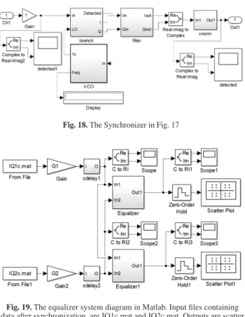
According to our previous experience, the equalizer can compensate small frequency differences. It follows the three PLLs can be decreased to two. In ideal case, 𝜔𝜔3= −𝜔𝜔1. 𝜔𝜔2= 𝜔𝜔1, and 𝜔𝜔4= −𝜔𝜔2. Thus, with two PLLs that are locked to the input carrier frequencies, the synchronization can be solved. Details are found on Fig. 16.
Fig. 16. Finding the proper LO frequencies at receiver side by use of two Costas loops. We use here our Costas loop
version that is suggested for large noise [6]
The synchronizer consists of two Costas loops, and the VCO drive signal is formulated from both complex inputs.
Realization of Fig. 16 in Matlab is presented in the next Figures that are found at the end of the paper. The detected I and Q signals are shown in Fig. 20.
Then the details of the equalizer follow. The equalizer is a four-channel adaptive filter. Inputs of the equalizer are the complex signals from the synchronizer as shown in Fig. 16.
3
Fig. 7. The phase-frequency detector PFD in Fig. 6
Fig. 8. The VCO in Fig. 6
First we show how the pilot frequency is found.
Fig. 9. Initial transient in instantaneous frequency
Settling time is about 0.2 msec. Now the detected I and Q signals are filtered.
Fig. 10. The previous Figure, magnified. After settling, the frequency is kept within 1 kHz
Fig. 11. Filtering system
Fig. 12. Filter characteristics
As a conclusion of this example, a faster method is needed that is more accurate. Costas loop is too time-consuming.
Now we remove the pilot. The result is that the constellation diagram cannot be reconstructed in this way.
IV. themcmaequalIzerandplls
Detection of 2x2 MIMO signals INFOCOMMUNICATIONS JOURNAL
SEPTEMBER 2020 • VOLUME XII • NUMBER 3 27
Fig. 13. FFT of the received signal without a pilot
Fig. 14. The previous Figure, with increased frequency resolution
Fig. 15. The problem: The constellation diagram cannot be reconstructed in this way
4. The MCMA equalizer and PLLs
Basically, we have two problems. Deviation of the transmitted and received frequencies, and separation of the
way.
The baseband receiver signal 𝑥𝑥̂for perfect separation, can be formulated as follows:
𝑥𝑥̂ = 𝐴𝐴−1𝐻𝐻−1𝐵𝐵−1𝑟𝑟 =
= [𝑒𝑒−𝑗𝑗𝜔𝜔1𝑡𝑡 0
0 𝑒𝑒−𝑗𝑗𝜔𝜔2𝑡𝑡] [1/2 𝑗𝑗/2𝑗𝑗/2 1/2] [𝑒𝑒−𝑗𝑗𝜔𝜔3𝑡𝑡 0 0 𝑒𝑒−𝑗𝑗𝜔𝜔4𝑡𝑡] 𝑟𝑟
(8) where 𝜔𝜔1,𝜔𝜔2are the two LO frequencies at transmitter side and 𝜔𝜔3,𝜔𝜔4are the two LO frequencies at receiver side. In ideal case, 𝜔𝜔1= −𝜔𝜔3and 𝜔𝜔2= −𝜔𝜔4.
From our experiments we know that the equalizer can stop a slow rotation. For this reason, instead of Eq. (8), we may use
𝑥𝑥̂ =1𝑐𝑐𝐴𝐴−1𝐻𝐻−1𝑐𝑐𝐵𝐵−1𝑟𝑟 =
[1 0
0 𝑒𝑒−𝑗𝑗(𝜔𝜔2−𝜔𝜔1)𝑡𝑡] [1/2 𝑗𝑗/2𝑗𝑗/2 1/2] [𝑒𝑒−𝑗𝑗(𝜔𝜔3+𝜔𝜔1)𝑡𝑡 0 0 𝑒𝑒−𝑗𝑗(𝜔𝜔4+𝜔𝜔1)𝑡𝑡] 𝑟𝑟
(9) where 𝑐𝑐 = 𝑒𝑒−𝑗𝑗𝜔𝜔1𝑡𝑡. Consequently, three PLLs may solve the problem. One at the output of the equalizer with frequency 𝜔𝜔2− 𝜔𝜔1, and two before the equalizer with frequencies 𝜔𝜔3+ 𝜔𝜔1and 𝜔𝜔3+ 𝜔𝜔1.
According to our previous experience, the equalizer can compensate small frequency differences. It follows the three PLLs can be decreased to two. In ideal case, 𝜔𝜔3= −𝜔𝜔1. 𝜔𝜔2= 𝜔𝜔1, and 𝜔𝜔4= −𝜔𝜔2. Thus, with two PLLs that are locked to the input carrier frequencies, the synchronization can be solved. Details are found on Fig. 16.
Fig. 16. Finding the proper LO frequencies at receiver side by use of two Costas loops. We use here our Costas loop
version that is suggested for large noise [6]
The synchronizer consists of two Costas loops, and the VCO drive signal is formulated from both complex inputs.
Realization of Fig. 16 in Matlab is presented in the next Figures that are found at the end of the paper. The detected I and Q signals are shown in Fig. 20.
Then the details of the equalizer follow. The equalizer is a four-channel adaptive filter. Inputs of the equalizer are the complex signals from the synchronizer as shown in Fig. 16.
Fig. 13. FFT of the received signal without a pilot
Fig. 14. The previous Figure, with increased frequency resolution
Fig. 15. The problem: The constellation diagram cannot be reconstructed in this way
4. The MCMA equalizer and PLLs
Basically, we have two problems. Deviation of the transmitted and received frequencies, and separation of the
way.
The baseband receiver signal 𝑥𝑥̂for perfect separation, can be formulated as follows:
𝑥𝑥̂ = 𝐴𝐴−1𝐻𝐻−1𝐵𝐵−1𝑟𝑟 =
= [𝑒𝑒−𝑗𝑗𝜔𝜔1𝑡𝑡 0
0 𝑒𝑒−𝑗𝑗𝜔𝜔2𝑡𝑡] [1/2 𝑗𝑗/2𝑗𝑗/2 1/2] [𝑒𝑒−𝑗𝑗𝜔𝜔3𝑡𝑡 0 0 𝑒𝑒−𝑗𝑗𝜔𝜔4𝑡𝑡] 𝑟𝑟
(8) where 𝜔𝜔1,𝜔𝜔2are the two LO frequencies at transmitter side and 𝜔𝜔3,𝜔𝜔4are the two LO frequencies at receiver side. In ideal case, 𝜔𝜔1= −𝜔𝜔3and 𝜔𝜔2= −𝜔𝜔4.
From our experiments we know that the equalizer can stop a slow rotation. For this reason, instead of Eq. (8), we may use
𝑥𝑥̂ =1𝑐𝑐𝐴𝐴−1𝐻𝐻−1𝑐𝑐𝐵𝐵−1𝑟𝑟 =
[1 0
0 𝑒𝑒−𝑗𝑗(𝜔𝜔2−𝜔𝜔1)𝑡𝑡] [1/2 𝑗𝑗/2𝑗𝑗/2 1/2] [𝑒𝑒−𝑗𝑗(𝜔𝜔3+𝜔𝜔1)𝑡𝑡 0 0 𝑒𝑒−𝑗𝑗(𝜔𝜔4+𝜔𝜔1)𝑡𝑡] 𝑟𝑟
(9) where 𝑐𝑐 = 𝑒𝑒−𝑗𝑗𝜔𝜔1𝑡𝑡. Consequently, three PLLs may solve the problem. One at the output of the equalizer with frequency 𝜔𝜔2− 𝜔𝜔1, and two before the equalizer with frequencies 𝜔𝜔3+ 𝜔𝜔1and 𝜔𝜔3+ 𝜔𝜔1.
According to our previous experience, the equalizer can compensate small frequency differences. It follows the three PLLs can be decreased to two. In ideal case, 𝜔𝜔3= −𝜔𝜔1. 𝜔𝜔2= 𝜔𝜔1, and 𝜔𝜔4= −𝜔𝜔2. Thus, with two PLLs that are locked to the input carrier frequencies, the synchronization can be solved. Details are found on Fig. 16.
Fig. 16. Finding the proper LO frequencies at receiver side by use of two Costas loops. We use here our Costas loop
version that is suggested for large noise [6]
The synchronizer consists of two Costas loops, and the VCO drive signal is formulated from both complex inputs.
Realization of Fig. 16 in Matlab is presented in the next Figures that are found at the end of the paper. The detected I and Q signals are shown in Fig. 20.
Then the details of the equalizer follow. The equalizer is a four-channel adaptive filter. Inputs of the equalizer are the complex signals from the synchronizer as shown in Fig. 16.
4
Fig. 13. FFT of the received signal without a pilot
Fig. 14. The previous Figure, with increased frequency resolution
Fig. 15. The problem: The constellation diagram cannot be reconstructed in this way
4. The MCMA equalizer and PLLs
Basically, we have two problems. Deviation of the transmitted and received frequencies, and separation of the
two transmitted signals at receiver side. Deviation is solved by PLLs, separation and signal equalization are solved by adaptive filters. Deviation can be modelled in the following way.
The baseband receiver signal 𝑥𝑥̂for perfect separation, can be formulated as follows:
𝑥𝑥̂ = 𝐴𝐴−1𝐻𝐻−1𝐵𝐵−1𝑟𝑟 =
= [𝑒𝑒−𝑗𝑗𝜔𝜔1𝑡𝑡 0
0 𝑒𝑒−𝑗𝑗𝜔𝜔2𝑡𝑡] [1/2 𝑗𝑗/2𝑗𝑗/2 1/2] [𝑒𝑒−𝑗𝑗𝜔𝜔3𝑡𝑡 0 0 𝑒𝑒−𝑗𝑗𝜔𝜔4𝑡𝑡] 𝑟𝑟
(8) where 𝜔𝜔1,𝜔𝜔2are the two LO frequencies at transmitter side and 𝜔𝜔3,𝜔𝜔4are the two LO frequencies at receiver side. In ideal case, 𝜔𝜔1= −𝜔𝜔3and 𝜔𝜔2= −𝜔𝜔4.
From our experiments we know that the equalizer can stop a slow rotation. For this reason, instead of Eq. (8), we may use
𝑥𝑥̂ =1𝑐𝑐𝐴𝐴−1𝐻𝐻−1𝑐𝑐𝐵𝐵−1𝑟𝑟 =
[1 0
0 𝑒𝑒−𝑗𝑗(𝜔𝜔2−𝜔𝜔1)𝑡𝑡] [1/2 𝑗𝑗/2𝑗𝑗/2 1/2] [𝑒𝑒−𝑗𝑗(𝜔𝜔3+𝜔𝜔1)𝑡𝑡 0 0 𝑒𝑒−𝑗𝑗(𝜔𝜔4+𝜔𝜔1)𝑡𝑡] 𝑟𝑟
(9) where 𝑐𝑐 = 𝑒𝑒−𝑗𝑗𝜔𝜔1𝑡𝑡. Consequently, three PLLs may solve the problem. One at the output of the equalizer with frequency 𝜔𝜔2− 𝜔𝜔1, and two before the equalizer with frequencies 𝜔𝜔3+ 𝜔𝜔1and 𝜔𝜔3+ 𝜔𝜔1.
According to our previous experience, the equalizer can compensate small frequency differences. It follows the three PLLs can be decreased to two. In ideal case, 𝜔𝜔3= −𝜔𝜔1. 𝜔𝜔2= 𝜔𝜔1, and 𝜔𝜔4= −𝜔𝜔2. Thus, with two PLLs that are locked to the input carrier frequencies, the synchronization can be solved. Details are found on Fig. 16.
Fig. 16. Finding the proper LO frequencies at receiver side by use of two Costas loops. We use here our Costas loop
version that is suggested for large noise [6]
The synchronizer consists of two Costas loops, and the VCO drive signal is formulated from both complex inputs.
Realization of Fig. 16 in Matlab is presented in the next Figures that are found at the end of the paper. The detected I and Q signals are shown in Fig. 20.
Then the details of the equalizer follow. The equalizer is a four-channel adaptive filter. Inputs of the equalizer are the complex signals from the synchronizer as shown in Fig. 16.
5
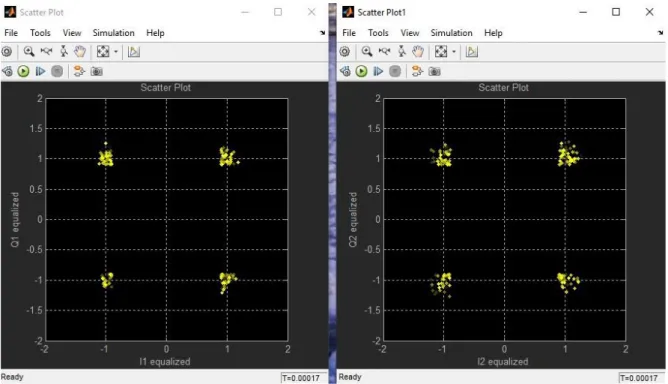
The system diagram of the equalizer are also found at the end of the paper.
Now the I and Q signals at both channels must be reconstructed. We use the MCMA (Modified constant modulus algorithm) [1]. Its essence is the following. The equalized signal is, according to Eq. (8):
𝑥𝑥̂1= 𝑤𝑤1𝑟𝑟1+ 𝑤𝑤2𝑟𝑟2 (10) 𝑥𝑥̂2= 𝑤𝑤3𝑟𝑟1+ 𝑤𝑤4𝑟𝑟2 (11) where 𝑤𝑤𝑖𝑖-s are the weight factors of the adaptive filter channels. Initial values are 𝑤𝑤1,1= 𝑤𝑤4,1=12, 𝑤𝑤2,1= 𝑤𝑤3,1=
1
2𝑗𝑗,according to Eq. (9). A possible choice would be 𝑤𝑤1= 𝑤𝑤4and 𝑤𝑤2= 𝑤𝑤3. This would require an ideal placement of the antennas at vertices of a rectangle. But this rectangle may be distorted by several reasons resulting in hurting condition 𝑤𝑤2= 𝑤𝑤3.
Change of the equalized signals is
∆𝑥𝑥̂1= ∆𝑤𝑤1𝑟𝑟1+ 𝑤𝑤1∆𝑟𝑟1+ ∆𝑤𝑤2𝑟𝑟2+𝑤𝑤2∆𝑟𝑟2 (12)
∆𝑥𝑥̂2= ∆𝑤𝑤3𝑟𝑟1+ 𝑤𝑤3∆𝑟𝑟1+ ∆𝑤𝑤4𝑟𝑟2+𝑤𝑤4∆𝑟𝑟2 (13) where ∆𝑤𝑤1,𝑘𝑘 = 𝑤𝑤1,𝑘𝑘− 𝑤𝑤1,𝑘𝑘−1 in the kth iteration, and similarly for the other weight factors. The signals in the next iteration are 𝑥𝑥̂1+ ∆𝑥𝑥̂1 and 𝑥𝑥̂2+ ∆𝑥𝑥̂2. The error signals are defined as
𝜀𝜀1= {𝑥𝑥̂1,1}(|𝑥𝑥̂1,1| − 𝑅𝑅1) + 𝑗𝑗{𝑥𝑥̂1,2}(|𝑥𝑥̂1,2| − 𝑅𝑅2) (14) 𝜀𝜀2= {𝑥𝑥̂2,1}(|𝑥𝑥̂2,1| − 𝑅𝑅1) + 𝑗𝑗{𝑥𝑥̂2,2}(|𝑥𝑥̂1,2| − 𝑅𝑅2) (15) where the complex radius of the constellation diagram is 𝑅𝑅 = 𝑅𝑅1+ 𝑗𝑗𝑅𝑅2= |𝑅𝑅|(1 + 𝑗𝑗)/√2, braces denote signum, and 𝑟𝑟1= 𝑥𝑥̂1,1+ 𝑗𝑗𝑥𝑥̂1,2. The goal is 𝜀𝜀1= 𝑚𝑚𝑚𝑚𝑚𝑚. and 𝜀𝜀2= 𝑚𝑚𝑚𝑚𝑚𝑚.
Changes of the equalized signals are
∆𝑥𝑥̂1= −𝜇𝜇1𝜀𝜀1 (16)
∆𝑥𝑥̂2= −𝜇𝜇2𝜀𝜀2 (17)
where∆denotes the change during the last sampling period.
From Eq. (12, 13) changes of the weight factors during the last sampling period are
[∆𝑤𝑤∆𝑤𝑤12] = [𝑟𝑟1 𝑟𝑟2]+ (∆𝑥𝑥̂1− 𝑤𝑤1∆𝑟𝑟1− 𝑤𝑤2∆𝑟𝑟2) (18) [∆𝑤𝑤∆𝑤𝑤34] = [𝑟𝑟1 𝑟𝑟2]+ (∆𝑥𝑥̂2− 𝑤𝑤3∆𝑟𝑟1− 𝑤𝑤4∆𝑟𝑟2) (19) in the kth iteration, where + denotes Moore-Penrose generalized inverse. Here we exploit the fact that the generalized inverse gives the minimum norm solution of an under-determined system [10].
The algorithm starts with 𝑤𝑤1,𝑤𝑤2,𝑤𝑤3,𝑤𝑤4,𝑟𝑟1and 𝑟𝑟2. Then Eq. (10, 11, 14-19) are executed. Then w-s and r-s are delayed. Similarly, for the other channel. The given algorithm significantly differs from known algorithms [1].
Robustness of the algorithm has been observed during all runs.
5. Related questions
Here we summarize some other important ideas related to 2 x 2 MIMO detection.
Filter method
Essence of the filter method is that instead of a PLL, a filter is applied for synchronization. Advantage with respect to the previous Chapter is, that the random changes on LO frequencies are much smaller, and locking problems are eliminated. Hardware requirements are of the same amount.
FFT method
The filter function can be realized by applying FFT of the input signal. FFT is computation consuming, so it is a hard decision how often the FFT is made. Advantages are the same as for the filter method.
False detection cancellation
False detection occurs when the received constellation diagram suddenly rotates by 90°. Originally, we made a great effort on false detection cancellation. However, in our previous publication [8], we pointed out that the most efficient solution of this problem is application of differential coding. Thus, we omit here the list of other methods for false detection cancellation.
The 1-bit method [9]
The main difference between this and our method is that in this method, the signal after synchronization is digitized. This is a limiting case, in the literature few bits A/D conversion can also be found. The author’s opinion is that the possible advantage of decreasing the noise effects is virtual, because it remains at the random variation of zero crossings. Moreover, strong learning algorithms may be needed for equalization that are time consuming.
More than 4 antennas
In case of more than 4 antennas, differences in distances between a transmitter antenna and neighboring receiver antennas cannot be kept constant. Even synchronization is more difficult, because there are many transmitter frequencies that can be different all. Equalization is to invert the matrix describing the relation between separate transmitter and receiver signals. But these are possible [3], however, the extra advantage of more than 4 antennas decrease.
Higher order modulation
Essentially arbitrary order (power of 2) can be used [4].
In our opinion, its significance is not too high because for higher order modulation, noise sensitivity rapidly increases, and it is a better solution to apply lower order modulation at higher speed.
6. Conclusions
The synchronization by two Costas loops and the equalization using an adaptive filter have been detailed. The